Parallel computing with Dask#
Xarray integrates with Dask to support parallel computations and streaming computation on datasets that don’t fit into memory. Currently, Dask is an entirely optional feature for xarray. However, the benefits of using Dask are sufficiently strong that Dask may become a required dependency in a future version of xarray.
For a full example of how to use xarray’s Dask integration, read the blog post introducing xarray and Dask. More up-to-date examples may be found at the Pangeo project’s gallery and at the Dask examples website.
What is a Dask array?#
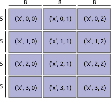
Dask divides arrays into many small pieces, called chunks, each of which is presumed to be small enough to fit into memory.
Unlike NumPy, which has eager evaluation, operations on Dask arrays are lazy. Operations queue up a series of tasks mapped over blocks, and no computation is performed until you actually ask values to be computed (e.g., to print results to your screen or write to disk). At that point, data is loaded into memory and computation proceeds in a streaming fashion, block-by-block.
The actual computation is controlled by a multi-processing or thread pool, which allows Dask to take full advantage of multiple processors available on most modern computers.
For more details, read the Dask documentation.
Note that xarray only makes use of dask.array and dask.delayed.
Reading and writing data#
The usual way to create a Dataset filled with Dask arrays is to load the
data from a netCDF file or files. You can do this by supplying a chunks
argument to open_dataset() or using the
open_mfdataset() function.
In [1]: ds = xr.open_dataset("example-data.nc", chunks={"time": 10})

In [2]: ds
Out[2]:
<xarray.Dataset> Size: 8MB
Dimensions:      (time: 30, latitude: 180, longitude: 180)
Coordinates:
  * time         (time) datetime64[ns] 240B 2015-01-01 2015-01-02 ... 2015-01-30
  * longitude    (longitude) int64 1kB 0 1 2 3 4 5 6 ... 174 175 176 177 178 179
  * latitude     (latitude) float64 1kB 89.5 88.5 87.5 ... -87.5 -88.5 -89.5
Data variables:
    temperature  (time, latitude, longitude) float64 8MB dask.array<chunksize=(10, 180, 180), meta=np.ndarray>
In this example latitude and longitude do not appear in the chunks
dict, so only one chunk will be used along those dimensions. It is also
entirely equivalent to opening a dataset using open_dataset()
and then chunking the data using the chunk method, e.g.,
xr.open_dataset('example-data.nc').chunk({'time': 10}).
To open multiple files simultaneously in parallel using Dask delayed,
use open_mfdataset():
xr.open_mfdataset('my/files/*.nc', parallel=True)
This function will automatically concatenate and merge datasets into one in
the simple cases that it understands (see combine_by_coords()
for the full disclaimer). By default, open_mfdataset() will chunk each
netCDF file into a single Dask array; again, supply the chunks argument to
control the size of the resulting Dask arrays. In more complex cases, you can
open each file individually using open_dataset() and merge the result, as
described in Combining data. Passing the keyword argument parallel=True to
open_mfdataset() will speed up the reading of large multi-file datasets by
executing those read tasks in parallel using dask.delayed.
Warning
open_mfdataset() called without chunks argument will return
dask arrays with chunk sizes equal to the individual files. Re-chunking
the dataset after creation with ds.chunk() will lead to an ineffective use of
memory and is not recommended.
You’ll notice that printing a dataset still shows a preview of array values, even if they are actually Dask arrays. We can do this quickly with Dask because we only need to compute the first few values (typically from the first block). To reveal the true nature of an array, print a DataArray:
In [3]: ds.temperature
Out[3]:
<xarray.DataArray 'temperature' (time: 30, latitude: 180, longitude: 180)> Size: 8MB
dask.array<open_dataset-temperature, shape=(30, 180, 180), dtype=float64, chunksize=(10, 180, 180), chunktype=numpy.ndarray>
Coordinates:
  * time       (time) datetime64[ns] 240B 2015-01-01 2015-01-02 ... 2015-01-30
  * longitude  (longitude) int64 1kB 0 1 2 3 4 5 6 ... 174 175 176 177 178 179
  * latitude   (latitude) float64 1kB 89.5 88.5 87.5 86.5 ... -87.5 -88.5 -89.5
Once you’ve manipulated a Dask array, you can still write a dataset too big to
fit into memory back to disk by using to_netcdf() in the
usual way.
In [4]: ds.to_netcdf("manipulated-example-data.nc")
By setting the compute argument to False, to_netcdf()
will return a dask.delayed object that can be computed later.
In [5]: from dask.diagnostics import ProgressBar

# or distributed.progress when using the distributed scheduler
In [6]: delayed_obj = ds.to_netcdf("manipulated-example-data.nc", compute=False)

In [7]: with ProgressBar():
   ...:     results = delayed_obj.compute()
   ...:

[                                        ] | 0% Completed | 116.36 us
[########################################] | 100% Completed | 100.32 ms
Note
When using Dask’s distributed scheduler to write NETCDF4 files, it may be necessary to set the environment variable HDF5_USE_FILE_LOCKING=FALSE to avoid competing locks within the HDF5 SWMR file locking scheme. Note that writing netCDF files with Dask’s distributed scheduler is only supported for the netcdf4 backend.
A dataset can also be converted to a Dask DataFrame using to_dask_dataframe().
In [8]: df = ds.to_dask_dataframe()

In [9]: df
Out[9]:
Dask DataFrame Structure:
                         time latitude longitude temperature
npartitions=3
0              datetime64[ns]  float64     int64     float64
324000                    ...      ...       ...         ...
648000                    ...      ...       ...         ...
971999                    ...      ...       ...         ...
Dask Name: concat, 5 expressions
Expr=Concat(frames=[FromGraph(db8dc53), FromGraph(96b8cd6), FromGraph(3b4dfe1), FromGraph(7ba0c2b)], axis=1)
Dask DataFrames do not support multi-indexes so the coordinate variables from the dataset are included as columns in the Dask DataFrame.
Using Dask with xarray#
Nearly all existing xarray methods (including those for indexing, computation, concatenating and grouped operations) have been extended to work automatically with Dask arrays. When you load data as a Dask array in an xarray data structure, almost all xarray operations will keep it as a Dask array; when this is not possible, they will raise an exception rather than unexpectedly loading data into memory. Converting a Dask array into memory generally requires an explicit conversion step. One notable exception is indexing operations: to enable label based indexing, xarray will automatically load coordinate labels into memory.
Tip
By default, dask uses its multi-threaded scheduler, which distributes work across multiple cores and allows for processing some datasets that do not fit into memory. For running across a cluster, setup the distributed scheduler.
The easiest way to convert an xarray data structure from lazy Dask arrays into
eager, in-memory NumPy arrays is to use the load() method:
In [10]: ds.load()
Out[10]:
<xarray.Dataset> Size: 8MB
Dimensions:      (time: 30, latitude: 180, longitude: 180)
Coordinates:
  * time         (time) datetime64[ns] 240B 2015-01-01 2015-01-02 ... 2015-01-30
  * longitude    (longitude) int64 1kB 0 1 2 3 4 5 6 ... 174 175 176 177 178 179
  * latitude     (latitude) float64 1kB 89.5 88.5 87.5 ... -87.5 -88.5 -89.5
Data variables:
    temperature  (time, latitude, longitude) float64 8MB 0.4691 ... -0.2467
You can also access values, which will always be a
NumPy array:
In [11]: ds.temperature.values
Out[11]:
array([[[  4.691e-01,  -2.829e-01, ...,  -5.577e-01,   3.814e-01],
        [  1.337e+00,  -1.531e+00, ...,   8.726e-01,  -1.538e+00],
        ...
# truncated for brevity
Explicit conversion by wrapping a DataArray with np.asarray also works:
In [12]: np.asarray(ds.temperature)
Out[12]:
array([[[  4.691e-01,  -2.829e-01, ...,  -5.577e-01,   3.814e-01],
        [  1.337e+00,  -1.531e+00, ...,   8.726e-01,  -1.538e+00],
        ...
Alternatively you can load the data into memory but keep the arrays as
Dask arrays using the persist() method:
In [13]: persisted = ds.persist()
persist() is particularly useful when using a
distributed cluster because the data will be loaded into distributed memory
across your machines and be much faster to use than reading repeatedly from
disk.
Warning
On a single machine persist() will try to load all of
your data into memory. You should make sure that your dataset is not larger than
available memory.
Note
For more on the differences between persist() and
compute() see this Stack Overflow answer on the differences between client persist and client compute and the Dask documentation.
For performance you may wish to consider chunk sizes. The correct choice of
chunk size depends both on your data and on the operations you want to perform.
With xarray, both converting data to a Dask arrays and converting the chunk
sizes of Dask arrays is done with the chunk() method:
In [14]: rechunked = ds.chunk({"latitude": 100, "longitude": 100})
Warning
Rechunking an existing dask array created with open_mfdataset()
is not recommended (see above).
You can view the size of existing chunks on an array by viewing the
chunks attribute:
In [15]: rechunked.chunks
Out[15]: Frozen({'time': (30,), 'latitude': (100, 80), 'longitude': (100, 80)})
If there are not consistent chunksizes between all the arrays in a dataset
along a particular dimension, an exception is raised when you try to access
.chunks.
Note
In the future, we would like to enable automatic alignment of Dask chunksizes (but not the other way around). We might also require that all arrays in a dataset share the same chunking alignment. Neither of these are currently done.
NumPy ufuncs like np.sin transparently work on all xarray objects, including those
that store lazy Dask arrays:
In [16]: import numpy as np

In [17]: np.sin(rechunked)
Out[17]:
<xarray.Dataset> Size: 8MB
Dimensions:      (time: 30, latitude: 180, longitude: 180)
Coordinates:
  * time         (time) datetime64[ns] 240B 2015-01-01 2015-01-02 ... 2015-01-30
  * longitude    (longitude) int64 1kB 0 1 2 3 4 5 6 ... 174 175 176 177 178 179
  * latitude     (latitude) float64 1kB 89.5 88.5 87.5 ... -87.5 -88.5 -89.5
Data variables:
    temperature  (time, latitude, longitude) float64 8MB dask.array<chunksize=(30, 100, 100), meta=np.ndarray>
To access Dask arrays directly, use the
DataArray.data attribute. This attribute exposes
array data either as a Dask array or as a NumPy array, depending on whether it has been
loaded into Dask or not:
In [18]: ds.temperature.data
Out[18]:
array([[[ 4.691e-01, -2.829e-01, -1.509e+00, ..., -8.584e-01,  3.070e-01, -2.867e-02],
        [ 3.843e-01,  1.574e+00,  1.589e+00, ..., -7.983e-01, -5.577e-01,  3.814e-01],
        [ 1.337e+00, -1.531e+00,  1.331e+00, ...,  1.116e+00, -4.439e-01, -2.005e-01],
        ...,
        [-9.767e-01,  1.153e+00,  2.368e-01, ..., -2.358e+00,  7.173e-01, -3.645e-01],
        [-4.878e-01,  3.862e-01,  6.693e-02, ...,  1.047e+00,  1.519e+00,  1.234e+00],
        [ 8.305e-01,  3.307e-01, -7.652e-03, ...,  3.320e-01,  6.742e-01, -6.534e-01]],

       [[ 1.830e-01, -1.192e+00, -8.357e-02, ...,  3.961e-01,  2.800e-01, -7.277e-01],
        [ 2.057e+00, -1.163e+00,  2.464e-01, ...,  6.132e-01, -8.074e-01,  1.021e+00],
        [-4.868e-01,  7.992e-02,  9.419e-01, ..., -8.465e-01,  2.024e-01, -8.869e-01],
        ...,
        [ 1.137e-01, -6.739e-01, -6.066e-03, ..., -2.464e-01, -8.723e-01, -5.857e-01],
        [ 1.871e-01,  8.154e-02,  2.765e-01, ...,  3.445e-01, -1.893e-01, -2.018e-01],
        [ 8.611e-01,  1.849e+00,  9.102e-01, ..., -9.998e-01,  2.341e+00,  1.089e+00]],

       [[-9.274e-01,  1.177e+00,  5.248e-01, ...,  1.319e+00,  1.202e+00,  5.705e-02],
        [ 1.753e+00, -2.929e-01,  1.585e+00, ..., -3.762e-01,  4.622e-01,  1.767e+00],
        [ 9.798e-04, -1.524e-01, -9.568e-02, ..., -1.023e+00, -5.611e-01, -1.384e+00],
        ...,
        [-1.355e-01, -1.741e+00, -3.228e-02, ..., -1.431e-01, -1.546e+00, -5.870e-01],
        [-1.192e-01,  1.063e+00, -4.556e-02, ...,  1.547e+00,  1.188e+00,  1.530e-01],
        [ 8.955e-01, -1.530e+00, -1.375e+00, ..., -5.880e-01,  2.055e+00,  2.625e+00]],

       ...,

       [[ 1.465e+00, -1.316e+00,  4.056e-02, ...,  5.967e-01, -1.001e+00, -9.458e-02],
        [-1.961e+00, -1.458e+00, -1.366e+00, ..., -2.769e-01, -7.274e-01,  1.925e-01],
        [ 5.085e-03, -1.558e+00, -5.966e-01, ..., -2.901e-01, -6.704e-01, -1.495e+00],
        ...,
        [-2.026e-01,  6.837e-01,  5.485e-01, ...,  2.302e-02, -1.714e+00,  1.224e+00],
        [ 6.145e-01,  8.913e-01,  1.595e+00, ..., -1.572e+00,  2.206e+00,  1.441e-01],
        [ 8.968e-01, -1.058e-02,  1.375e+00, ...,  1.326e+00, -1.596e+00,  1.755e+00]],

       [[ 2.798e-01, -1.042e+00, -9.158e-01, ...,  1.105e+00, -4.097e-01,  6.651e-01],
        [-1.821e-01, -1.315e+00, -3.048e-01, ...,  1.280e-01, -1.776e+00, -1.208e+00],
        [-7.035e-01, -5.634e-01,  1.499e+00, ..., -2.037e-01, -1.552e-01, -1.001e+00],
        ...,
        [-4.242e-01, -3.481e-01, -4.598e-01, ..., -1.912e+00,  8.812e-01,  8.306e-01],
        [-1.766e+00, -7.101e-01, -3.624e-02, ...,  1.893e+00, -4.464e-02, -3.418e-01],
        [-4.511e-01, -9.322e-01,  5.886e-01, ...,  9.546e-01, -1.616e+00,  5.361e-01]],

       [[ 1.827e+00,  1.758e-01, -3.515e-01, ..., -5.171e-01, -3.210e-01,  3.487e-02],
        [ 1.296e+00, -9.241e-01, -4.683e-01, ..., -1.143e+00,  5.967e-01,  4.978e-01],
        [-2.550e-01,  1.545e+00, -1.851e+00, ...,  1.141e+00, -8.020e-01,  1.415e+00],
        ...,
        [ 9.623e-01, -1.391e+00,  7.754e-01, ...,  7.441e-01,  1.019e+00,  6.441e-02],
        [ 1.650e-02, -5.006e-01, -7.921e-01, ...,  2.091e+00, -8.625e-01,  7.333e-01],
        [-1.472e+00,  6.782e-01, -1.407e+00, ...,  8.119e-01, -2.485e-01, -2.467e-01]]])
Note
.data is also used to expose other “computable” array backends beyond Dask and
NumPy (e.g. sparse and pint arrays).
Automatic parallelization with apply_ufunc and map_blocks#
Almost all of xarray’s built-in operations work on Dask arrays. If you want to use a function that isn’t wrapped by xarray, and have it applied in parallel on each block of your xarray object, you have three options:
Extract Dask arrays from xarray objects (
.data) and use Dask directly.Use
apply_ufunc()to apply functions that consume and return NumPy arrays.Use
map_blocks(),Dataset.map_blocks()orDataArray.map_blocks()to apply functions that consume and return xarray objects.
apply_ufunc#
apply_ufunc() automates embarrassingly parallel “map” type operations
where a function written for processing NumPy arrays should be repeatedly
applied to xarray objects containing Dask arrays. It works similarly to
dask.array.map_blocks() and dask.array.blockwise(), but without
requiring an intermediate layer of abstraction.
For the best performance when using Dask’s multi-threaded scheduler, wrap a function that already releases the global interpreter lock, which fortunately already includes most NumPy and Scipy functions. Here we show an example using NumPy operations and a fast function from bottleneck, which we use to calculate Spearman’s rank-correlation coefficient:
import numpy as np
import xarray as xr
import bottleneck


def covariance_gufunc(x, y):
    return (
        (x - x.mean(axis=-1, keepdims=True)) * (y - y.mean(axis=-1, keepdims=True))
    ).mean(axis=-1)


def pearson_correlation_gufunc(x, y):
    return covariance_gufunc(x, y) / (x.std(axis=-1) * y.std(axis=-1))


def spearman_correlation_gufunc(x, y):
    x_ranks = bottleneck.rankdata(x, axis=-1)
    y_ranks = bottleneck.rankdata(y, axis=-1)
    return pearson_correlation_gufunc(x_ranks, y_ranks)


def spearman_correlation(x, y, dim):
    return xr.apply_ufunc(
        spearman_correlation_gufunc,
        x,
        y,
        input_core_dims=[[dim], [dim]],
        dask="parallelized",
        output_dtypes=[float],
    )
The only aspect of this example that is different from standard usage of
apply_ufunc() is that we needed to supply the output_dtypes arguments.
(Read up on Wrapping custom computation for an explanation of the
“core dimensions” listed in input_core_dims.)
Our new spearman_correlation() function achieves near linear speedup
when run on large arrays across the four cores on my laptop. It would also
work as a streaming operation, when run on arrays loaded from disk:
In [19]: rs = np.random.RandomState(0)

In [20]: array1 = xr.DataArray(rs.randn(1000, 100000), dims=["place", "time"])  # 800MB

In [21]: array2 = array1 + 0.5 * rs.randn(1000, 100000)

# using one core, on NumPy arrays
In [22]: %time _ = spearman_correlation(array1, array2, 'time')
CPU times: user 21.6 s, sys: 2.84 s, total: 24.5 s
Wall time: 24.9 s

In [23]: chunked1 = array1.chunk({"place": 10})

In [24]: chunked2 = array2.chunk({"place": 10})

# using all my laptop's cores, with Dask
In [25]: r = spearman_correlation(chunked1, chunked2, "time").compute()

In [26]: %time _ = r.compute()
CPU times: user 30.9 s, sys: 1.74 s, total: 32.6 s
Wall time: 4.59 s
One limitation of apply_ufunc() is that it cannot be applied to arrays with
multiple chunks along a core dimension:
In [27]: spearman_correlation(chunked1, chunked2, "place")
ValueError: dimension 'place' on 0th function argument to apply_ufunc with
dask='parallelized' consists of multiple chunks, but is also a core
dimension. To fix, rechunk into a single Dask array chunk along this
dimension, i.e., ``.rechunk({'place': -1})``, but beware that this may
significantly increase memory usage.
This reflects the nature of core dimensions, in contrast to broadcast (non-core) dimensions that allow operations to be split into arbitrary chunks for application.
Tip
For the majority of NumPy functions that are already wrapped by Dask, it’s
usually a better idea to use the pre-existing dask.array function, by
using either a pre-existing xarray methods or
apply_ufunc() with dask='allowed'. Dask can often
have a more efficient implementation that makes use of the specialized
structure of a problem, unlike the generic speedups offered by
dask='parallelized'.
map_blocks#
Functions that consume and return xarray objects can be easily applied in parallel using map_blocks().
Your function will receive an xarray Dataset or DataArray subset to one chunk
along each chunked dimension.
In [28]: ds.temperature
Out[28]:
<xarray.DataArray 'temperature' (time: 30, latitude: 180, longitude: 180)> Size: 8MB
array([[[ 4.691e-01, -2.829e-01, -1.509e+00, ..., -8.584e-01,  3.070e-01, -2.867e-02],
        [ 3.843e-01,  1.574e+00,  1.589e+00, ..., -7.983e-01, -5.577e-01,  3.814e-01],
        [ 1.337e+00, -1.531e+00,  1.331e+00, ...,  1.116e+00, -4.439e-01, -2.005e-01],
        ...,
        [-9.767e-01,  1.153e+00,  2.368e-01, ..., -2.358e+00,  7.173e-01, -3.645e-01],
        [-4.878e-01,  3.862e-01,  6.693e-02, ...,  1.047e+00,  1.519e+00,  1.234e+00],
        [ 8.305e-01,  3.307e-01, -7.652e-03, ...,  3.320e-01,  6.742e-01, -6.534e-01]],

       [[ 1.830e-01, -1.192e+00, -8.357e-02, ...,  3.961e-01,  2.800e-01, -7.277e-01],
        [ 2.057e+00, -1.163e+00,  2.464e-01, ...,  6.132e-01, -8.074e-01,  1.021e+00],
        [-4.868e-01,  7.992e-02,  9.419e-01, ..., -8.465e-01,  2.024e-01, -8.869e-01],
        ...,
        [ 1.137e-01, -6.739e-01, -6.066e-03, ..., -2.464e-01, -8.723e-01, -5.857e-01],
        [ 1.871e-01,  8.154e-02,  2.765e-01, ...,  3.445e-01, -1.893e-01, -2.018e-01],
        [ 8.611e-01,  1.849e+00,  9.102e-01, ..., -9.998e-01,  2.341e+00,  1.089e+00]],

       [[-9.274e-01,  1.177e+00,  5.248e-01, ...,  1.319e+00,  1.202e+00,  5.705e-02],
        [ 1.753e+00, -2.929e-01,  1.585e+00, ..., -3.762e-01,  4.622e-01,  1.767e+00],
        [ 9.798e-04, -1.524e-01, -9.568e-02, ..., -1.023e+00, -5.611e-01, -1.384e+00],
        ...,
...
        ...,
        [-2.026e-01,  6.837e-01,  5.485e-01, ...,  2.302e-02, -1.714e+00,  1.224e+00],
        [ 6.145e-01,  8.913e-01,  1.595e+00, ..., -1.572e+00,  2.206e+00,  1.441e-01],
        [ 8.968e-01, -1.058e-02,  1.375e+00, ...,  1.326e+00, -1.596e+00,  1.755e+00]],

       [[ 2.798e-01, -1.042e+00, -9.158e-01, ...,  1.105e+00, -4.097e-01,  6.651e-01],
        [-1.821e-01, -1.315e+00, -3.048e-01, ...,  1.280e-01, -1.776e+00, -1.208e+00],
        [-7.035e-01, -5.634e-01,  1.499e+00, ..., -2.037e-01, -1.552e-01, -1.001e+00],
        ...,
        [-4.242e-01, -3.481e-01, -4.598e-01, ..., -1.912e+00,  8.812e-01,  8.306e-01],
        [-1.766e+00, -7.101e-01, -3.624e-02, ...,  1.893e+00, -4.464e-02, -3.418e-01],
        [-4.511e-01, -9.322e-01,  5.886e-01, ...,  9.546e-01, -1.616e+00,  5.361e-01]],

       [[ 1.827e+00,  1.758e-01, -3.515e-01, ..., -5.171e-01, -3.210e-01,  3.487e-02],
        [ 1.296e+00, -9.241e-01, -4.683e-01, ..., -1.143e+00,  5.967e-01,  4.978e-01],
        [-2.550e-01,  1.545e+00, -1.851e+00, ...,  1.141e+00, -8.020e-01,  1.415e+00],
        ...,
        [ 9.623e-01, -1.391e+00,  7.754e-01, ...,  7.441e-01,  1.019e+00,  6.441e-02],
        [ 1.650e-02, -5.006e-01, -7.921e-01, ...,  2.091e+00, -8.625e-01,  7.333e-01],
        [-1.472e+00,  6.782e-01, -1.407e+00, ...,  8.119e-01, -2.485e-01, -2.467e-01]]])
Coordinates:
  * time       (time) datetime64[ns] 240B 2015-01-01 2015-01-02 ... 2015-01-30
  * longitude  (longitude) int64 1kB 0 1 2 3 4 5 6 ... 174 175 176 177 178 179
  * latitude   (latitude) float64 1kB 89.5 88.5 87.5 86.5 ... -87.5 -88.5 -89.5
This DataArray has 3 chunks each with length 10 along the time dimension.
At compute time, a function applied with map_blocks() will receive a DataArray corresponding to a single block of shape 10x180x180
(time x latitude x longitude) with values loaded. The following snippet illustrates how to check the shape of the object
received by the applied function.
In [29]: def func(da):
   ....:     print(da.sizes)
   ....:     return da.time
   ....:

In [30]: mapped = xr.map_blocks(func, ds.temperature)
Frozen({'time': 30, 'latitude': 180, 'longitude': 180})

In [31]: mapped
Out[31]:
<xarray.DataArray 'time' (time: 30)> Size: 240B
array(['2015-01-01T00:00:00.000000000', '2015-01-02T00:00:00.000000000',
       '2015-01-03T00:00:00.000000000', '2015-01-04T00:00:00.000000000',
       '2015-01-05T00:00:00.000000000', '2015-01-06T00:00:00.000000000',
       '2015-01-07T00:00:00.000000000', '2015-01-08T00:00:00.000000000',
       '2015-01-09T00:00:00.000000000', '2015-01-10T00:00:00.000000000',
       '2015-01-11T00:00:00.000000000', '2015-01-12T00:00:00.000000000',
       '2015-01-13T00:00:00.000000000', '2015-01-14T00:00:00.000000000',
       '2015-01-15T00:00:00.000000000', '2015-01-16T00:00:00.000000000',
       '2015-01-17T00:00:00.000000000', '2015-01-18T00:00:00.000000000',
       '2015-01-19T00:00:00.000000000', '2015-01-20T00:00:00.000000000',
       '2015-01-21T00:00:00.000000000', '2015-01-22T00:00:00.000000000',
       '2015-01-23T00:00:00.000000000', '2015-01-24T00:00:00.000000000',
       '2015-01-25T00:00:00.000000000', '2015-01-26T00:00:00.000000000',
       '2015-01-27T00:00:00.000000000', '2015-01-28T00:00:00.000000000',
       '2015-01-29T00:00:00.000000000', '2015-01-30T00:00:00.000000000'],
      dtype='datetime64[ns]')
Coordinates:
  * time     (time) datetime64[ns] 240B 2015-01-01 2015-01-02 ... 2015-01-30
Notice that the map_blocks() call printed
Frozen({'time': 0, 'latitude': 0, 'longitude': 0}) to screen.
func is received 0-sized blocks! map_blocks() needs to know what the final result
looks like in terms of dimensions, shapes etc. It does so by running the provided function on 0-shaped
inputs (automated inference). This works in many cases, but not all. If automatic inference does not
work for your function, provide the template kwarg (see below).
In this case, automatic inference has worked so let’s check that the result is as expected.
In [32]: mapped.load(scheduler="single-threaded")
Out[32]:
<xarray.DataArray 'time' (time: 30)> Size: 240B
array(['2015-01-01T00:00:00.000000000', '2015-01-02T00:00:00.000000000',
       '2015-01-03T00:00:00.000000000', '2015-01-04T00:00:00.000000000',
       '2015-01-05T00:00:00.000000000', '2015-01-06T00:00:00.000000000',
       '2015-01-07T00:00:00.000000000', '2015-01-08T00:00:00.000000000',
       '2015-01-09T00:00:00.000000000', '2015-01-10T00:00:00.000000000',
       '2015-01-11T00:00:00.000000000', '2015-01-12T00:00:00.000000000',
       '2015-01-13T00:00:00.000000000', '2015-01-14T00:00:00.000000000',
       '2015-01-15T00:00:00.000000000', '2015-01-16T00:00:00.000000000',
       '2015-01-17T00:00:00.000000000', '2015-01-18T00:00:00.000000000',
       '2015-01-19T00:00:00.000000000', '2015-01-20T00:00:00.000000000',
       '2015-01-21T00:00:00.000000000', '2015-01-22T00:00:00.000000000',
       '2015-01-23T00:00:00.000000000', '2015-01-24T00:00:00.000000000',
       '2015-01-25T00:00:00.000000000', '2015-01-26T00:00:00.000000000',
       '2015-01-27T00:00:00.000000000', '2015-01-28T00:00:00.000000000',
       '2015-01-29T00:00:00.000000000', '2015-01-30T00:00:00.000000000'],
      dtype='datetime64[ns]')
Coordinates:
  * time     (time) datetime64[ns] 240B 2015-01-01 2015-01-02 ... 2015-01-30

In [33]: mapped.identical(ds.time)
Out[33]: True
Note that we use .load(scheduler="single-threaded") to execute the computation.
This executes the Dask graph in serial using a for loop, but allows for printing to screen and other
debugging techniques. We can easily see that our function is receiving blocks of shape 10x180x180 and
the returned result is identical to ds.time as expected.
Here is a common example where automated inference will not work.
In [34]: def func(da):
   ....:     print(da.sizes)
   ....:     return da.isel(time=[1])
   ....:

In [35]: mapped = xr.map_blocks(func, ds.temperature)
Frozen({'time': 30, 'latitude': 180, 'longitude': 180})
func cannot be run on 0-shaped inputs because it is not possible to extract element 1 along a
dimension of size 0. In this case we need to tell map_blocks() what the returned result looks
like using the template kwarg. template must be an xarray Dataset or DataArray (depending on
what the function returns) with dimensions, shapes, chunk sizes, attributes, coordinate variables and data
variables that look exactly like the expected result. The variables should be dask-backed and hence not
incur much memory cost.
Note
Note that when template is provided, attrs from template are copied over to the result. Any
attrs set in func will be ignored.
In [36]: template = ds.temperature.isel(time=[1, 11, 21])

In [37]: mapped = xr.map_blocks(func, ds.temperature, template=template)
Frozen({'time': 30, 'latitude': 180, 'longitude': 180})
Notice that the 0-shaped sizes were not printed to screen. Since template has been provided
map_blocks() does not need to infer it by running func on 0-shaped inputs.
In [38]: mapped.identical(template)
Out[38]: False
map_blocks() also allows passing args and kwargs down to the user function func.
func will be executed as func(block_xarray, *args, **kwargs) so args must be a list and kwargs must be a dictionary.
In [39]: def func(obj, a, b=0):
   ....:     return obj + a + b
   ....:

In [40]: mapped = ds.map_blocks(func, args=[10], kwargs={"b": 10})

In [41]: expected = ds + 10 + 10

In [42]: mapped.identical(expected)
Out[42]: True
Tip
As map_blocks() loads each block into memory, reduce as much as possible objects consumed by user functions.
For example, drop useless variables before calling func with map_blocks().
Chunking and performance#
The chunks parameter has critical performance implications when using Dask
arrays. If your chunks are too small, queueing up operations will be extremely
slow, because Dask will translate each operation into a huge number of
operations mapped across chunks. Computation on Dask arrays with small chunks
can also be slow, because each operation on a chunk has some fixed overhead from
the Python interpreter and the Dask task executor.
Conversely, if your chunks are too big, some of your computation may be wasted, because Dask only computes results one chunk at a time.
A good rule of thumb is to create arrays with a minimum chunksize of at least one million elements (e.g., a 1000x1000 matrix). With large arrays (10+ GB), the cost of queueing up Dask operations can be noticeable, and you may need even larger chunksizes.
Tip
Check out the dask documentation on chunks.
Optimization Tips#
With analysis pipelines involving both spatial subsetting and temporal resampling, Dask performance can become very slow or memory hungry in certain cases. Here are some optimization tips we have found through experience:
Do your spatial and temporal indexing (e.g.
.sel()or.isel()) early in the pipeline, especially before callingresample()orgroupby(). Grouping and resampling triggers some computation on all the blocks, which in theory should commute with indexing, but this optimization hasn’t been implemented in Dask yet. (See Dask issue #746).More generally,
groupby()is a costly operation and will perform a lot better if thefloxpackage is installed. See the flox documentation for more. By default Xarray will usefloxif installed.Save intermediate results to disk as a netCDF files (using
to_netcdf()) and then load them again withopen_dataset()for further computations. For example, if subtracting temporal mean from a dataset, save the temporal mean to disk before subtracting. Again, in theory, Dask should be able to do the computation in a streaming fashion, but in practice this is a fail case for the Dask scheduler, because it tries to keep every chunk of an array that it computes in memory. (See Dask issue #874)Specify smaller chunks across space when using
open_mfdataset()(e.g.,chunks={'latitude': 10, 'longitude': 10}). This makes spatial subsetting easier, because there’s no risk you will load subsets of data which span multiple chunks. On individual files, prefer to subset before chunking (suggestion 1).Chunk as early as possible, and avoid rechunking as much as possible. Always pass the
chunks={}argument toopen_mfdataset()to avoid redundant file reads.Using the h5netcdf package by passing
engine='h5netcdf'toopen_mfdataset()can be quicker than the defaultengine='netcdf4'that uses the netCDF4 package.Find best practices specific to Dask arrays in the documentation.
The dask diagnostics can be useful in identifying performance bottlenecks.