You can run this notebook in a live session ![]() or view it on Github.
or view it on Github.
Calculating Seasonal Averages from Time Series of Monthly Means#
Author: Joe Hamman
The data used for this example can be found in the xarray-data repository. You may need to change the path to rasm.nc below.
Suppose we have a netCDF or xarray.Dataset of monthly mean data and we want to calculate the seasonal average. To do this properly, we need to calculate the weighted average considering that each month has a different number of days.
[1]:
%matplotlib inline
import numpy as np
import pandas as pd
import xarray as xr
import matplotlib.pyplot as plt
Open the Dataset#
[2]:
ds = xr.tutorial.open_dataset("rasm").load()
ds
[2]:
<xarray.Dataset> Size: 17MB
Dimensions:  (time: 36, y: 205, x: 275)
Coordinates:
  * time     (time) object 288B 1980-09-16 12:00:00 ... 1983-08-17 00:00:00
    xc       (y, x) float64 451kB 189.2 189.4 189.6 189.7 ... 17.4 17.15 16.91
    yc       (y, x) float64 451kB 16.53 16.78 17.02 17.27 ... 28.01 27.76 27.51
Dimensions without coordinates: y, x
Data variables:
    Tair     (time, y, x) float64 16MB nan nan nan nan ... 28.66 28.19 28.21
Attributes:
    title:                     /workspace/jhamman/processed/R1002RBRxaaa01a/l...
    institution:               U.W.
    source:                    RACM R1002RBRxaaa01a
    output_frequency:          daily
    output_mode:               averaged
    convention:                CF-1.4
    references:                Based on the initial model of Liang et al., 19...
    comment:                   Output from the Variable Infiltration Capacity...
    nco_openmp_thread_number:  1
    NCO:                       netCDF Operators version 4.7.9 (Homepage = htt...
history: Fri Aug 7 17:57:38 2020: ncatted -a bounds,,d...Now for the heavy lifting:#
We first have to come up with the weights, - calculate the month length for each monthly data record - calculate weights using groupby('time.season')
Finally, we just need to multiply our weights by the Dataset and sum along the time dimension. Creating a DataArray for the month length is as easy as using the days_in_month accessor on the time coordinate. The calendar type, in this case 'noleap', is automatically considered in this operation.
[3]:
month_length = ds.time.dt.days_in_month
month_length
[3]:
<xarray.DataArray 'days_in_month' (time: 36)> Size: 288B
array([30, 31, 30, 31, 31, 28, 31, 30, 31, 30, 31, 31, 30, 31, 30, 31, 31, 28,
       31, 30, 31, 30, 31, 31, 30, 31, 30, 31, 31, 28, 31, 30, 31, 30, 31, 31])
Coordinates:
  * time     (time) object 288B 1980-09-16 12:00:00 ... 1983-08-17 00:00:00
Attributes:
    long_name:       time
type_preferred: int[4]:
# Calculate the weights by grouping by 'time.season'.
weights = (
    month_length.groupby("time.season") / month_length.groupby("time.season").sum()
)

# Test that the sum of the weights for each season is 1.0
np.testing.assert_allclose(weights.groupby("time.season").sum().values, np.ones(4))

# Calculate the weighted average
ds_weighted = (ds * weights).groupby("time.season").sum(dim="time")
[5]:
ds_weighted
[5]:
<xarray.Dataset> Size: 3MB
Dimensions:  (y: 205, x: 275, season: 4)
Coordinates:
    xc       (y, x) float64 451kB 189.2 189.4 189.6 189.7 ... 17.4 17.15 16.91
    yc       (y, x) float64 451kB 16.53 16.78 17.02 17.27 ... 28.01 27.76 27.51
  * season   (season) object 32B 'DJF' 'JJA' 'MAM' 'SON'
Dimensions without coordinates: y, x
Data variables:
Tair (season, y, x) float64 2MB 0.0 0.0 0.0 0.0 ... 22.08 21.73 21.96[6]:
# only used for comparisons
ds_unweighted = ds.groupby("time.season").mean("time")
ds_diff = ds_weighted - ds_unweighted
[7]:
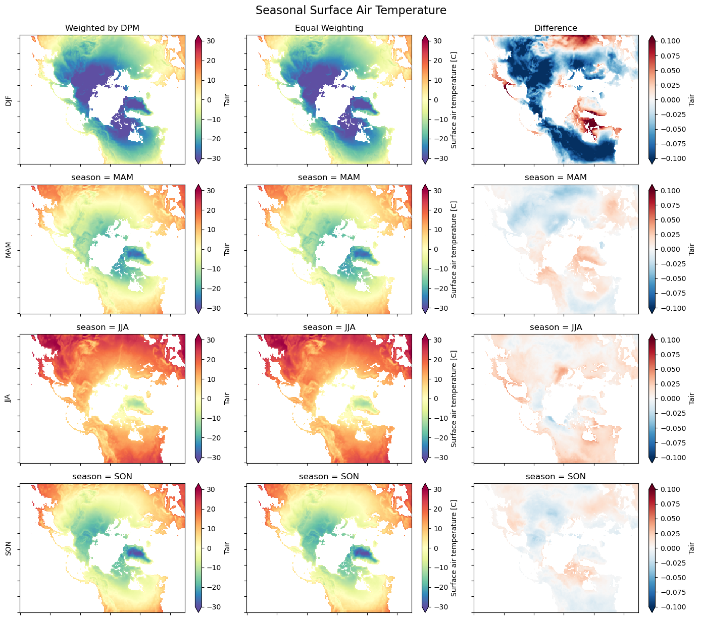
# Quick plot to show the results
notnull = pd.notnull(ds_unweighted["Tair"][0])

fig, axes = plt.subplots(nrows=4, ncols=3, figsize=(14, 12))
for i, season in enumerate(("DJF", "MAM", "JJA", "SON")):
    ds_weighted["Tair"].sel(season=season).where(notnull).plot.pcolormesh(
        ax=axes[i, 0],
        vmin=-30,
        vmax=30,
        cmap="Spectral_r",
        add_colorbar=True,
        extend="both",
    )

    ds_unweighted["Tair"].sel(season=season).where(notnull).plot.pcolormesh(
        ax=axes[i, 1],
        vmin=-30,
        vmax=30,
        cmap="Spectral_r",
        add_colorbar=True,
        extend="both",
    )

    ds_diff["Tair"].sel(season=season).where(notnull).plot.pcolormesh(
        ax=axes[i, 2],
        vmin=-0.1,
        vmax=0.1,
        cmap="RdBu_r",
        add_colorbar=True,
        extend="both",
    )

    axes[i, 0].set_ylabel(season)
    axes[i, 1].set_ylabel("")
    axes[i, 2].set_ylabel("")

for ax in axes.flat:
    ax.axes.get_xaxis().set_ticklabels([])
    ax.axes.get_yaxis().set_ticklabels([])
    ax.axes.axis("tight")
    ax.set_xlabel("")

axes[0, 0].set_title("Weighted by DPM")
axes[0, 1].set_title("Equal Weighting")
axes[0, 2].set_title("Difference")

plt.tight_layout()

fig.suptitle("Seasonal Surface Air Temperature", fontsize=16, y=1.02)
[7]:
Text(0.5, 1.02, 'Seasonal Surface Air Temperature')
[8]:
# Wrap it into a simple function
def season_mean(ds, calendar="standard"):
    # Make a DataArray with the number of days in each month, size = len(time)
    month_length = ds.time.dt.days_in_month

    # Calculate the weights by grouping by 'time.season'
    weights = (
        month_length.groupby("time.season") / month_length.groupby("time.season").sum()
    )

    # Test that the sum of the weights for each season is 1.0
    np.testing.assert_allclose(weights.groupby("time.season").sum().values, np.ones(4))

    # Calculate the weighted average
    return (ds * weights).groupby("time.season").sum(dim="time")