You can run this notebook in a live session ![]() or view it on Github.
or view it on Github.
Toy weather data#
Here is an example of how to easily manipulate a toy weather dataset using xarray and other recommended Python libraries:
[1]:
import numpy as np
import pandas as pd
import seaborn as sns

import xarray as xr

np.random.seed(123)

xr.set_options(display_style="html")

times = pd.date_range("2000-01-01", "2001-12-31", name="time")
annual_cycle = np.sin(2 * np.pi * (times.dayofyear.values / 365.25 - 0.28))

base = 10 + 15 * annual_cycle.reshape(-1, 1)
tmin_values = base + 3 * np.random.randn(annual_cycle.size, 3)
tmax_values = base + 10 + 3 * np.random.randn(annual_cycle.size, 3)

ds = xr.Dataset(
    {
        "tmin": (("time", "location"), tmin_values),
        "tmax": (("time", "location"), tmax_values),
    },
    {"time": times, "location": ["IA", "IN", "IL"]},
)

ds
[1]:
<xarray.Dataset> Size: 41kB
Dimensions:   (time: 731, location: 3)
Coordinates:
  * time      (time) datetime64[ns] 6kB 2000-01-01 2000-01-02 ... 2001-12-31
  * location  (location) <U2 24B 'IA' 'IN' 'IL'
Data variables:
    tmin      (time, location) float64 18kB -8.037 -1.788 ... -1.346 -4.544
tmax (time, location) float64 18kB 12.98 3.31 6.779 ... 3.343 3.805Examine a dataset with pandas and seaborn#
Convert to a pandas DataFrame#
[2]:
df = ds.to_dataframe()
df.head()
[2]:
| tmin | tmax | ||
|---|---|---|---|
| time | location | ||
| 2000-01-01 | IA | -8.037369 | 12.980549 |
| IN | -1.788441 | 3.310409 | |
| IL | -3.931542 | 6.778554 | |
| 2000-01-02 | IA | -9.341157 | 0.447856 |
| IN | -6.558073 | 6.372712 |
[3]:
df.describe()
[3]:
| tmin | tmax | |
|---|---|---|
| count | 2193.000000 | 2193.000000 |
| mean | 9.975426 | 20.108232 |
| std | 10.963228 | 11.010569 |
| min | -13.395763 | -3.506234 |
| 25% | -0.040347 | 9.853905 |
| 50% | 10.060403 | 19.967409 |
| 75% | 20.083590 | 30.045588 |
| max | 33.456060 | 43.271148 |
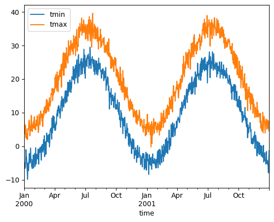
Visualize using pandas#
[4]:
ds.mean(dim="location").to_dataframe().plot()
[4]:
<Axes: xlabel='time'>
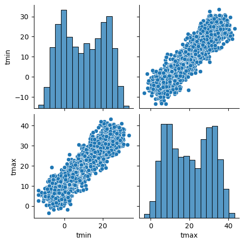
Visualize using seaborn#
[5]:
sns.pairplot(df.reset_index(), vars=ds.data_vars)
[5]:
<seaborn.axisgrid.PairGrid at 0x7ffbe08f7100>
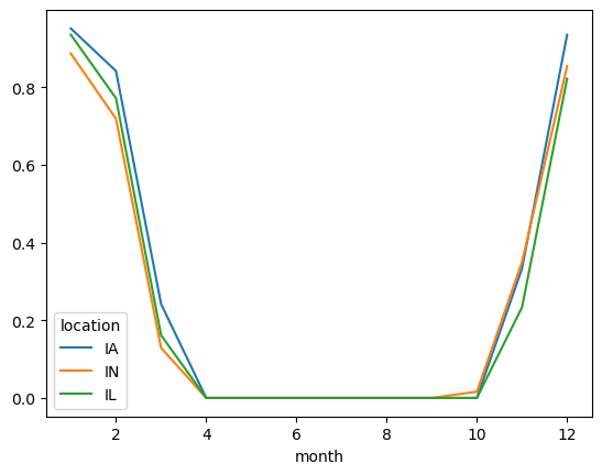
Probability of freeze by calendar month#
[6]:
freeze = (ds["tmin"] <= 0).groupby("time.month").mean("time")
freeze
[6]:
<xarray.DataArray 'tmin' (month: 12, location: 3)> Size: 288B
array([[0.9516129 , 0.88709677, 0.93548387],
       [0.84210526, 0.71929825, 0.77192982],
       [0.24193548, 0.12903226, 0.16129032],
       [0.        , 0.        , 0.        ],
       [0.        , 0.        , 0.        ],
       [0.        , 0.        , 0.        ],
       [0.        , 0.        , 0.        ],
       [0.        , 0.        , 0.        ],
       [0.        , 0.        , 0.        ],
       [0.        , 0.01612903, 0.        ],
       [0.33333333, 0.35      , 0.23333333],
       [0.93548387, 0.85483871, 0.82258065]])
Coordinates:
  * location  (location) <U2 24B 'IA' 'IN' 'IL'
* month (month) int64 96B 1 2 3 4 5 6 7 8 9 10 11 12[7]:
freeze.to_pandas().plot()
[7]:
<Axes: xlabel='month'>
Monthly averaging#
[8]:
monthly_avg = ds.resample(time="1MS").mean()
monthly_avg.sel(location="IA").to_dataframe().plot(style="s-")
[8]:
<Axes: xlabel='time'>
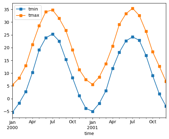
Note that MS here refers to Month-Start; M labels Month-End (the last day of the month).
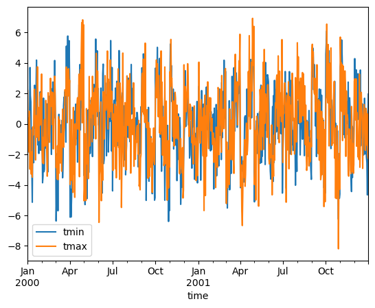
Calculate monthly anomalies#
In climatology, “anomalies” refer to the difference between observations and typical weather for a particular season. Unlike observations, anomalies should not show any seasonal cycle.
[9]:
climatology = ds.groupby("time.month").mean("time")
anomalies = ds.groupby("time.month") - climatology
anomalies.mean("location").to_dataframe()[["tmin", "tmax"]].plot()
[9]:
<Axes: xlabel='time'>
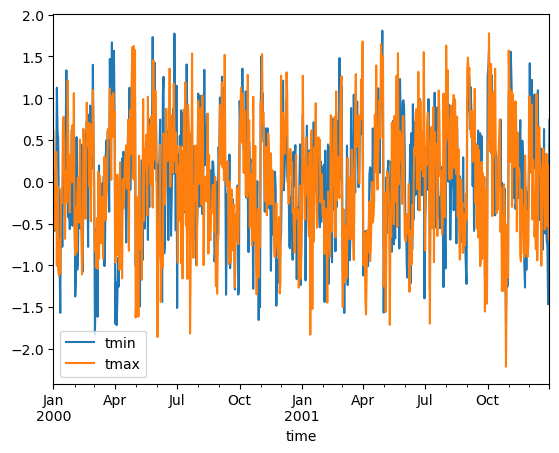
Calculate standardized monthly anomalies#
You can create standardized anomalies where the difference between the observations and the climatological monthly mean is divided by the climatological standard deviation.
[10]:
climatology_mean = ds.groupby("time.month").mean("time")
climatology_std = ds.groupby("time.month").std("time")
stand_anomalies = xr.apply_ufunc(
    lambda x, m, s: (x - m) / s,
    ds.groupby("time.month"),
    climatology_mean,
    climatology_std,
)

stand_anomalies.mean("location").to_dataframe()[["tmin", "tmax"]].plot()
[10]:
<Axes: xlabel='time'>
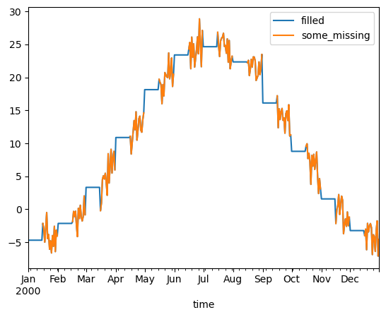
Fill missing values with climatology#
The fillna method on grouped objects lets you easily fill missing values by group:
[11]:
# throw away the first half of every month
some_missing = ds.tmin.sel(time=ds["time.day"] > 15).reindex_like(ds)
filled = some_missing.groupby("time.month").fillna(climatology.tmin)
both = xr.Dataset({"some_missing": some_missing, "filled": filled})
both
[11]:
<xarray.Dataset> Size: 47kB
Dimensions:       (time: 731, location: 3)
Coordinates:
  * time          (time) datetime64[ns] 6kB 2000-01-01 2000-01-02 ... 2001-12-31
  * location      (location) <U2 24B 'IA' 'IN' 'IL'
    month         (time) int64 6kB 1 1 1 1 1 1 1 1 1 ... 12 12 12 12 12 12 12 12
Data variables:
    some_missing  (time, location) float64 18kB nan nan nan ... -1.346 -4.544
filled (time, location) float64 18kB -5.163 -4.216 ... -1.346 -4.544[12]:
df = both.sel(time="2000").mean("location").reset_coords(drop=True).to_dataframe()
df.head()
[12]:
| some_missing | filled | |
|---|---|---|
| time | ||
| 2000-01-01 | NaN | -4.686763 |
| 2000-01-02 | NaN | -4.686763 |
| 2000-01-03 | NaN | -4.686763 |
| 2000-01-04 | NaN | -4.686763 |
| 2000-01-05 | NaN | -4.686763 |
[13]:
df[["filled", "some_missing"]].plot()
[13]:
<Axes: xlabel='time'>