You can run this notebook in a live session ![]() or view it on Github.
or view it on Github.
GRIB Data Example#
GRIB format is commonly used to disseminate atmospheric model data. With xarray and the cfgrib engine, GRIB data can easily be analyzed and visualized.
[1]:
import xarray as xr
import matplotlib.pyplot as plt
To read GRIB data, you can use xarray.load_dataset. The only extra code you need is to specify the engine as cfgrib.
[2]:
ds = xr.tutorial.load_dataset("era5-2mt-2019-03-uk.grib", engine="cfgrib")
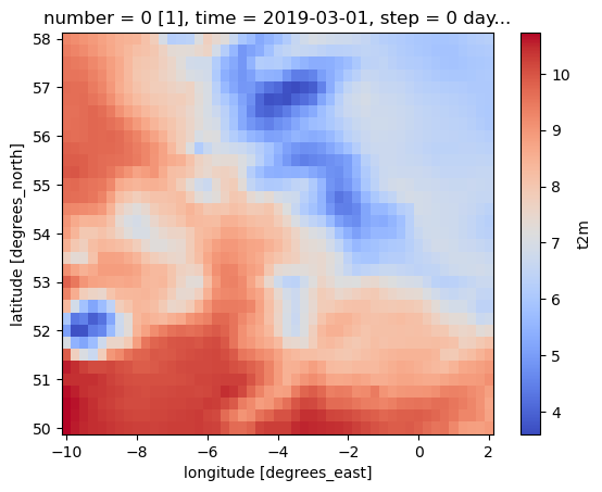
Let’s create a simple plot of 2-m air temperature in degrees Celsius:
[3]:
ds = ds - 273.15
ds.t2m[0].plot(cmap=plt.cm.coolwarm)
[3]:
<matplotlib.collections.QuadMesh at 0x7fdd832ed2d0>
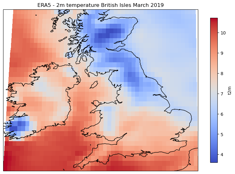
With CartoPy, we can create a more detailed plot, using built-in shapefiles to help provide geographic context:
[4]:
import cartopy.crs as ccrs
import cartopy

fig = plt.figure(figsize=(10, 10))
ax = plt.axes(projection=ccrs.Robinson())
ax.coastlines(resolution="10m")
plot = ds.t2m[0].plot(
    cmap=plt.cm.coolwarm, transform=ccrs.PlateCarree(), cbar_kwargs={"shrink": 0.6}
)
plt.title("ERA5 - 2m temperature British Isles March 2019")
[4]:
Text(0.5, 1.0, 'ERA5 - 2m temperature British Isles March 2019')
/home/docs/checkouts/readthedocs.org/user_builds/xray/conda/latest/lib/python3.10/site-packages/cartopy/io/__init__.py:241: DownloadWarning: Downloading: https://naturalearth.s3.amazonaws.com/10m_physical/ne_10m_coastline.zip
  warnings.warn(f'Downloading: {url}', DownloadWarning)
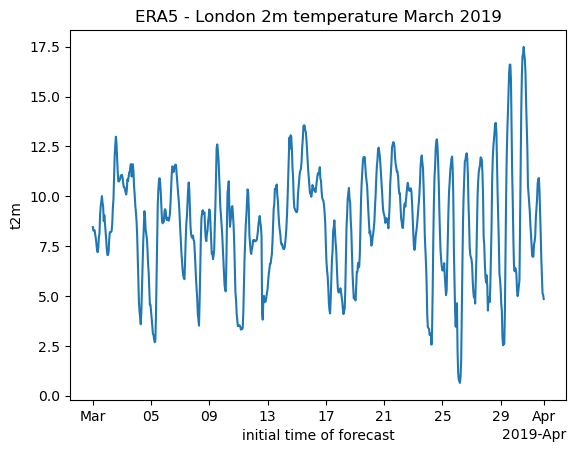
Finally, we can also pull out a time series for a given location easily:
[5]:
ds.t2m.sel(longitude=0, latitude=51.5).plot()
plt.title("ERA5 - London 2m temperature March 2019")
[5]:
Text(0.5, 1.0, 'ERA5 - London 2m temperature March 2019')