You can run this notebook in a live session ![]() or view it on Github.
or view it on Github.
Table of Contents
1 Compare weighted and unweighted mean temperature
1.0.1 Data
1.0.2 Creating weights
1.0.3 Weighted mean
1.0.4 Plot: comparison with unweighted mean
Compare weighted and unweighted mean temperature
Author: Mathias Hauser
We use the air_temperature example dataset to calculate the area-weighted temperature over its domain. This dataset has a regular latitude/ longitude grid, thus the gridcell area decreases towards the pole. For this grid we can use the cosine of the latitude as proxy for the grid cell area.
[1]:
%matplotlib inline

import cartopy.crs as ccrs
import matplotlib.pyplot as plt
import numpy as np

import xarray as xr
Data
Load the data, convert to celsius, and resample to daily values
[2]:
ds = xr.tutorial.load_dataset("air_temperature")

# to celsius
air = ds.air - 273.15

# resample from 6-hourly to daily values
air = air.resample(time="D").mean()

air
[2]:
<xarray.DataArray 'air' (time: 730, lat: 25, lon: 53)>
array([[[-31.2775   , -30.849998 , -30.475002 , ..., -39.7775   ,
         -37.975    , -35.475002 ],
        [-28.575005 , -28.5775   , -28.874996 , ..., -41.9025   ,
         -40.324997 , -36.85     ],
        [-19.149998 , -19.927498 , -21.3275   , ..., -41.675    ,
         -39.454998 , -34.524998 ],
        ...,
        [ 23.15001  ,  22.824997 ,  22.849998 , ...,  22.747505 ,
          22.170013 ,  21.795006 ],
        [ 23.174995 ,  23.574997 ,  23.592514 , ...,  23.022507 ,
          22.850006 ,  22.397507 ],
        [ 23.470009 ,  23.845001 ,  23.950005 , ...,  23.872505 ,
          23.897507 ,  23.82251  ]],

       [[-29.550003 , -29.650005 , -29.849998 , ..., -34.177498 ,
         -32.3525   , -30.0775   ],
        [-25.3275   , -25.95     , -26.927498 , ..., -37.225    ,
         -36.552498 , -34.550003 ],
        [-19.627502 , -21.0775   , -22.852497 , ..., -35.452496 ,
         -34.277496 , -31.25     ],
...
        [ 23.215004 ,  22.265    ,  22.015007 , ...,  23.740005 ,
          23.195007 ,  22.195    ],
        [ 24.3675   ,  24.514992 ,  23.895012 , ...,  23.415    ,
          22.995003 ,  22.269997 ],
        [ 25.417496 ,  25.592499 ,  25.192497 , ...,  23.642502 ,
          23.190002 ,  22.720001 ]],

       [[-28.935001 , -29.535    , -30.385002 , ..., -29.410004 ,
         -28.960003 , -28.46     ],
        [-23.834995 , -24.060001 , -24.559998 , ..., -32.585    ,
         -31.635002 , -30.035004 ],
        [-10.209999 , -10.784988 , -11.434998 , ..., -33.684998 ,
         -31.035    , -27.135002 ],
        ...,
        [ 21.69001  ,  21.990005 ,  23.489998 , ...,  22.265007 ,
          22.015    ,  21.415009 ],
        [ 23.390007 ,  24.439995 ,  24.94001  , ...,  22.415009 ,
          22.315002 ,  21.640007 ],
        [ 24.840012 ,  25.590004 ,  25.54     , ...,  23.065002 ,
          22.715004 ,  22.390007 ]]], dtype=float32)
Coordinates:
  * time     (time) datetime64[ns] 2013-01-01 2013-01-02 ... 2014-12-31
  * lat      (lat) float32 75.0 72.5 70.0 67.5 65.0 ... 25.0 22.5 20.0 17.5 15.0
* lon (lon) float32 200.0 202.5 205.0 207.5 ... 322.5 325.0 327.5 330.0- time: 730
- lat: 25
- lon: 53
- -31.28 -30.85 -30.48 -30.15 -29.85 ... 24.01 23.89 23.07 22.72 22.39
array([[[-31.2775 , -30.849998 , -30.475002 , ..., -39.7775 , -37.975 , -35.475002 ], [-28.575005 , -28.5775 , -28.874996 , ..., -41.9025 , -40.324997 , -36.85 ], [-19.149998 , -19.927498 , -21.3275 , ..., -41.675 , -39.454998 , -34.524998 ], ..., [ 23.15001 , 22.824997 , 22.849998 , ..., 22.747505 , 22.170013 , 21.795006 ], [ 23.174995 , 23.574997 , 23.592514 , ..., 23.022507 , 22.850006 , 22.397507 ], [ 23.470009 , 23.845001 , 23.950005 , ..., 23.872505 , 23.897507 , 23.82251 ]], [[-29.550003 , -29.650005 , -29.849998 , ..., -34.177498 , -32.3525 , -30.0775 ], [-25.3275 , -25.95 , -26.927498 , ..., -37.225 , -36.552498 , -34.550003 ], [-19.627502 , -21.0775 , -22.852497 , ..., -35.452496 , -34.277496 , -31.25 ], ... [ 23.215004 , 22.265 , 22.015007 , ..., 23.740005 , 23.195007 , 22.195 ], [ 24.3675 , 24.514992 , 23.895012 , ..., 23.415 , 22.995003 , 22.269997 ], [ 25.417496 , 25.592499 , 25.192497 , ..., 23.642502 , 23.190002 , 22.720001 ]], [[-28.935001 , -29.535 , -30.385002 , ..., -29.410004 , -28.960003 , -28.46 ], [-23.834995 , -24.060001 , -24.559998 , ..., -32.585 , -31.635002 , -30.035004 ], [-10.209999 , -10.784988 , -11.434998 , ..., -33.684998 , -31.035 , -27.135002 ], ..., [ 21.69001 , 21.990005 , 23.489998 , ..., 22.265007 , 22.015 , 21.415009 ], [ 23.390007 , 24.439995 , 24.94001 , ..., 22.415009 , 22.315002 , 21.640007 ], [ 24.840012 , 25.590004 , 25.54 , ..., 23.065002 , 22.715004 , 22.390007 ]]], dtype=float32) - time(time)datetime64[ns]2013-01-01 ... 2014-12-31
array(['2013-01-01T00:00:00.000000000', '2013-01-02T00:00:00.000000000', '2013-01-03T00:00:00.000000000', ..., '2014-12-29T00:00:00.000000000', '2014-12-30T00:00:00.000000000', '2014-12-31T00:00:00.000000000'], dtype='datetime64[ns]') - lat(lat)float3275.0 72.5 70.0 ... 20.0 17.5 15.0
- standard_name :
- latitude
- long_name :
- Latitude
- units :
- degrees_north
- axis :
- Y
array([75. , 72.5, 70. , 67.5, 65. , 62.5, 60. , 57.5, 55. , 52.5, 50. , 47.5, 45. , 42.5, 40. , 37.5, 35. , 32.5, 30. , 27.5, 25. , 22.5, 20. , 17.5, 15. ], dtype=float32) - lon(lon)float32200.0 202.5 205.0 ... 327.5 330.0
- standard_name :
- longitude
- long_name :
- Longitude
- units :
- degrees_east
- axis :
- X
array([200. , 202.5, 205. , 207.5, 210. , 212.5, 215. , 217.5, 220. , 222.5,
       225. , 227.5, 230. , 232.5, 235. , 237.5, 240. , 242.5, 245. , 247.5,
       250. , 252.5, 255. , 257.5, 260. , 262.5, 265. , 267.5, 270. , 272.5,
       275. , 277.5, 280. , 282.5, 285. , 287.5, 290. , 292.5, 295. , 297.5,
       300. , 302.5, 305. , 307.5, 310. , 312.5, 315. , 317.5, 320. , 322.5,
       325. , 327.5, 330. ], dtype=float32)
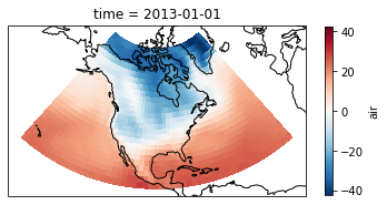
Plot the first timestep:
[3]:
projection = ccrs.LambertConformal(central_longitude=-95, central_latitude=45)

f, ax = plt.subplots(subplot_kw=dict(projection=projection))

air.isel(time=0).plot(transform=ccrs.PlateCarree(), cbar_kwargs=dict(shrink=0.7))
ax.coastlines()
[3]:
<cartopy.mpl.feature_artist.FeatureArtist at 0x7f735f1f3310>
Creating weights
For a rectangular grid the cosine of the latitude is proportional to the grid cell area.
[4]:
weights = np.cos(np.deg2rad(air.lat))
weights.name = "weights"
weights
[4]:
<xarray.DataArray 'weights' (lat: 25)>
array([0.25881907, 0.30070582, 0.34202015, 0.38268346, 0.42261827,
       0.4617486 , 0.49999997, 0.5372996 , 0.57357645, 0.6087614 ,
       0.6427876 , 0.67559016, 0.70710677, 0.7372773 , 0.76604444,
       0.7933533 , 0.81915206, 0.8433914 , 0.8660254 , 0.8870108 ,
       0.90630776, 0.9238795 , 0.9396926 , 0.95371693, 0.9659258 ],
      dtype=float32)
Coordinates:
  * lat      (lat) float32 75.0 72.5 70.0 67.5 65.0 ... 25.0 22.5 20.0 17.5 15.0
Attributes:
    standard_name:  latitude
    long_name:      Latitude
    units:          degrees_north
axis: Y- lat: 25
- 0.2588 0.3007 0.342 0.3827 0.4226 ... 0.9239 0.9397 0.9537 0.9659
array([0.25881907, 0.30070582, 0.34202015, 0.38268346, 0.42261827, 0.4617486 , 0.49999997, 0.5372996 , 0.57357645, 0.6087614 , 0.6427876 , 0.67559016, 0.70710677, 0.7372773 , 0.76604444, 0.7933533 , 0.81915206, 0.8433914 , 0.8660254 , 0.8870108 , 0.90630776, 0.9238795 , 0.9396926 , 0.95371693, 0.9659258 ], dtype=float32) - lat(lat)float3275.0 72.5 70.0 ... 20.0 17.5 15.0
- standard_name :
- latitude
- long_name :
- Latitude
- units :
- degrees_north
- axis :
- Y
array([75. , 72.5, 70. , 67.5, 65. , 62.5, 60. , 57.5, 55. , 52.5, 50. , 47.5,
       45. , 42.5, 40. , 37.5, 35. , 32.5, 30. , 27.5, 25. , 22.5, 20. , 17.5,
       15. ], dtype=float32)
- standard_name :
- latitude
- long_name :
- Latitude
- units :
- degrees_north
- axis :
- Y
Weighted mean
[5]:
air_weighted = air.weighted(weights)
air_weighted
[5]:
DataArrayWeighted with weights along dimensions: lat
[6]:
weighted_mean = air_weighted.mean(("lon", "lat"))
weighted_mean
[6]:
<xarray.DataArray (time: 730)>
array([ 6.092401 ,  5.5279922,  5.6512914,  5.786239 ,  5.9117665,
        5.6834373,  5.9767127,  6.456724 ,  6.5710645,  6.504647 ,
        6.134899 ,  5.926867 ,  5.8268237,  5.7228684,  5.5780067,
        5.4655232,  5.09124  ,  4.9860163,  5.22863  ,  5.2516627,
        5.4277263,  5.3877945,  5.4338994,  5.364401 ,  5.4685388,
        5.2290297,  5.350285 ,  5.3418307,  5.372671 ,  5.3595133,
        5.1403375,  5.0555673,  5.0724645,  5.23522  ,  5.3184857,
        5.4991755,  5.720886 ,  5.7286143,  5.7608094,  5.825561 ,
        6.268504 ,  6.436903 ,  6.510233 ,  6.564767 ,  6.6087847,
        6.4212685,  5.9147425,  5.5546775,  5.329217 ,  5.3359075,
        5.0705895,  5.283736 ,  5.5952206,  6.05466  ,  6.530731 ,
        6.507418 ,  6.3917418,  6.3951263,  6.3980885,  6.5293736,
        6.4771113,  6.535765 ,  6.692519 ,  6.6773686,  6.511633 ,
        6.4470334,  6.860378 ,  7.437535 ,  7.6981063,  7.484263 ,
        7.2581897,  7.135959 ,  7.093408 ,  7.267086 ,  7.348537 ,
        7.3217864,  7.221145 ,  7.212927 ,  7.2840424,  7.54338  ,
        7.854373 ,  8.11584  ,  8.261896 ,  8.111622 ,  8.219126 ,
        8.358713 ,  8.716147 ,  9.151885 ,  9.370043 ,  9.415865 ,
        9.073439 ,  8.820655 ,  8.804644 ,  8.856381 ,  9.0674515,
        9.40715  ,  9.696928 ,  9.742079 ,  9.659618 ,  9.695613 ,
...
       16.536924 , 16.133308 , 16.05551  , 16.100082 , 15.909406 ,
       15.764091 , 15.631487 , 15.827745 , 16.026222 , 16.319872 ,
       16.156448 , 15.898445 , 15.830862 , 15.810078 , 15.589792 ,
       15.309618 , 15.105176 , 14.96468  , 14.966973 , 14.904603 ,
       14.61066  , 14.330112 , 14.255611 , 14.31403  , 13.940103 ,
       13.758863 , 13.820865 , 14.021832 , 13.888187 , 13.724709 ,
       13.190875 , 12.995149 , 12.669842 , 12.585032 , 12.377669 ,
       12.178653 , 12.082313 , 11.874204 , 11.660166 , 11.601137 ,
       11.558611 , 11.183846 , 11.237345 , 11.091917 , 10.472193 ,
        9.898911 ,  9.431238 ,  9.491593 ,  9.688618 ,  9.998573 ,
        9.793551 ,  9.315285 ,  9.259933 ,  9.3849945,  9.343004 ,
        9.202585 ,  9.472328 ,  9.424212 ,  9.050674 ,  8.568184 ,
        7.7191467,  7.3312225,  7.4512987,  7.4235888,  7.518795 ,
        7.4950347,  7.623865 ,  8.083245 ,  8.049131 ,  8.027269 ,
        8.069612 ,  7.912531 ,  8.042945 ,  8.34481  ,  8.507071 ,
        8.708198 ,  8.604949 ,  8.312463 ,  8.257239 ,  7.9841394,
        7.693307 ,  7.421974 ,  7.4352374,  7.4829583,  7.642844 ,
        7.908468 ,  8.036132 ,  7.625418 ,  7.7533164,  7.850424 ,
        7.6213007,  6.8473396,  6.4502645,  5.985239 ,  5.5805774],
      dtype=float32)
Coordinates:
* time (time) datetime64[ns] 2013-01-01 2013-01-02 ... 2014-12-31- time: 730
- 6.092 5.528 5.651 5.786 5.912 5.683 ... 7.621 6.847 6.45 5.985 5.581
array([ 6.092401 , 5.5279922, 5.6512914, 5.786239 , 5.9117665, 5.6834373, 5.9767127, 6.456724 , 6.5710645, 6.504647 , 6.134899 , 5.926867 , 5.8268237, 5.7228684, 5.5780067, 5.4655232, 5.09124 , 4.9860163, 5.22863 , 5.2516627, 5.4277263, 5.3877945, 5.4338994, 5.364401 , 5.4685388, 5.2290297, 5.350285 , 5.3418307, 5.372671 , 5.3595133, 5.1403375, 5.0555673, 5.0724645, 5.23522 , 5.3184857, 5.4991755, 5.720886 , 5.7286143, 5.7608094, 5.825561 , 6.268504 , 6.436903 , 6.510233 , 6.564767 , 6.6087847, 6.4212685, 5.9147425, 5.5546775, 5.329217 , 5.3359075, 5.0705895, 5.283736 , 5.5952206, 6.05466 , 6.530731 , 6.507418 , 6.3917418, 6.3951263, 6.3980885, 6.5293736, 6.4771113, 6.535765 , 6.692519 , 6.6773686, 6.511633 , 6.4470334, 6.860378 , 7.437535 , 7.6981063, 7.484263 , 7.2581897, 7.135959 , 7.093408 , 7.267086 , 7.348537 , 7.3217864, 7.221145 , 7.212927 , 7.2840424, 7.54338 , 7.854373 , 8.11584 , 8.261896 , 8.111622 , 8.219126 , 8.358713 , 8.716147 , 9.151885 , 9.370043 , 9.415865 , 9.073439 , 8.820655 , 8.804644 , 8.856381 , 9.0674515, 9.40715 , 9.696928 , 9.742079 , 9.659618 , 9.695613 , ... 16.536924 , 16.133308 , 16.05551 , 16.100082 , 15.909406 , 15.764091 , 15.631487 , 15.827745 , 16.026222 , 16.319872 , 16.156448 , 15.898445 , 15.830862 , 15.810078 , 15.589792 , 15.309618 , 15.105176 , 14.96468 , 14.966973 , 14.904603 , 14.61066 , 14.330112 , 14.255611 , 14.31403 , 13.940103 , 13.758863 , 13.820865 , 14.021832 , 13.888187 , 13.724709 , 13.190875 , 12.995149 , 12.669842 , 12.585032 , 12.377669 , 12.178653 , 12.082313 , 11.874204 , 11.660166 , 11.601137 , 11.558611 , 11.183846 , 11.237345 , 11.091917 , 10.472193 , 9.898911 , 9.431238 , 9.491593 , 9.688618 , 9.998573 , 9.793551 , 9.315285 , 9.259933 , 9.3849945, 9.343004 , 9.202585 , 9.472328 , 9.424212 , 9.050674 , 8.568184 , 7.7191467, 7.3312225, 7.4512987, 7.4235888, 7.518795 , 7.4950347, 7.623865 , 8.083245 , 8.049131 , 8.027269 , 8.069612 , 7.912531 , 8.042945 , 8.34481 , 8.507071 , 8.708198 , 8.604949 , 8.312463 , 8.257239 , 7.9841394, 7.693307 , 7.421974 , 7.4352374, 7.4829583, 7.642844 , 7.908468 , 8.036132 , 7.625418 , 7.7533164, 7.850424 , 7.6213007, 6.8473396, 6.4502645, 5.985239 , 5.5805774], dtype=float32) - time(time)datetime64[ns]2013-01-01 ... 2014-12-31
array(['2013-01-01T00:00:00.000000000', '2013-01-02T00:00:00.000000000',
       '2013-01-03T00:00:00.000000000', ..., '2014-12-29T00:00:00.000000000',
       '2014-12-30T00:00:00.000000000', '2014-12-31T00:00:00.000000000'],
      dtype='datetime64[ns]')
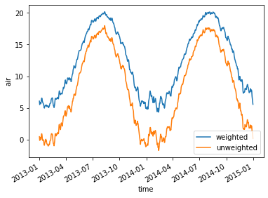
Plot: comparison with unweighted mean
Note how the weighted mean temperature is higher than the unweighted.
[7]:
weighted_mean.plot(label="weighted")
air.mean(("lon", "lat")).plot(label="unweighted")

plt.legend()
[7]:
<matplotlib.legend.Legend at 0x7f7360366460>