You can run this notebook in a live session ![]() or view it on Github.
or view it on Github.
Toy weather data
Here is an example of how to easily manipulate a toy weather dataset using xarray and other recommended Python libraries:
[1]:
import numpy as np
import pandas as pd
import seaborn as sns

import xarray as xr

np.random.seed(123)

xr.set_options(display_style="html")

times = pd.date_range("2000-01-01", "2001-12-31", name="time")
annual_cycle = np.sin(2 * np.pi * (times.dayofyear.values / 365.25 - 0.28))

base = 10 + 15 * annual_cycle.reshape(-1, 1)
tmin_values = base + 3 * np.random.randn(annual_cycle.size, 3)
tmax_values = base + 10 + 3 * np.random.randn(annual_cycle.size, 3)

ds = xr.Dataset(
    {
        "tmin": (("time", "location"), tmin_values),
        "tmax": (("time", "location"), tmax_values),
    },
    {"time": times, "location": ["IA", "IN", "IL"]},
)

ds
[1]:
xarray.Dataset
- location: 3
- time: 731
- time(time)datetime64[ns]2000-01-01 ... 2001-12-31
array(['2000-01-01T00:00:00.000000000', '2000-01-02T00:00:00.000000000', '2000-01-03T00:00:00.000000000', ..., '2001-12-29T00:00:00.000000000', '2001-12-30T00:00:00.000000000', '2001-12-31T00:00:00.000000000'], dtype='datetime64[ns]') - location(location)<U2'IA' 'IN' 'IL'
array(['IA', 'IN', 'IL'], dtype='<U2')
- tmin(time, location)float64-8.037 -1.788 ... -1.346 -4.544
array([[ -8.03736932, -1.78844117, -3.93154201], [ -9.34115662, -6.55807323, 0.13203714], [-12.13971902, -6.14641918, -1.06187252], ..., [ -5.34723825, -13.37459826, -4.93221199], [ -2.67283594, -5.18072141, -4.11567869], [ 2.06327582, -1.34576404, -4.54392729]]) - tmax(time, location)float6412.98 3.31 6.779 ... 3.343 3.805
array([[12.98054898,  3.31040942,  6.77855382],
       [ 0.44785582,  6.37271154,  4.8434966 ],
       [ 5.32269851,  6.25176289,  5.98033045],
       ...,
       [ 6.73078492,  7.74795302,  8.04569651],
       [ 6.46376911,  6.31695352,  1.55799171],
       [ 6.63593435,  3.34271537,  3.80527925]])
Examine a dataset with pandas and seaborn
Convert to a pandas DataFrame
[2]:
df = ds.to_dataframe()
df.head()
[2]:
| tmin | tmax | ||
|---|---|---|---|
| location | time | ||
| IA | 2000-01-01 | -8.037369 | 12.980549 |
| 2000-01-02 | -9.341157 | 0.447856 | |
| 2000-01-03 | -12.139719 | 5.322699 | |
| 2000-01-04 | -7.492914 | 1.889425 | |
| 2000-01-05 | -0.447129 | 0.791176 |
[3]:
df.describe()
[3]:
| tmin | tmax | |
|---|---|---|
| count | 2193.000000 | 2193.000000 |
| mean | 9.975426 | 20.108232 |
| std | 10.963228 | 11.010569 |
| min | -13.395763 | -3.506234 |
| 25% | -0.040347 | 9.853905 |
| 50% | 10.060403 | 19.967409 |
| 75% | 20.083590 | 30.045588 |
| max | 33.456060 | 43.271148 |
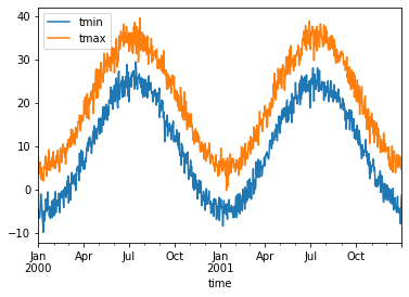
Visualize using pandas
[4]:
ds.mean(dim="location").to_dataframe().plot()
[4]:
<matplotlib.axes._subplots.AxesSubplot at 0x7f046d262280>
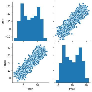
Visualize using seaborn
[5]:
sns.pairplot(df.reset_index(), vars=ds.data_vars)
[5]:
<seaborn.axisgrid.PairGrid at 0x7f046b16d7c0>
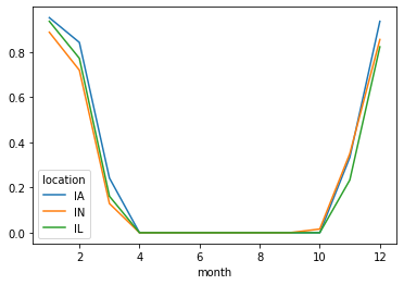
Probability of freeze by calendar month
[6]:
freeze = (ds["tmin"] <= 0).groupby("time.month").mean("time")
freeze
[6]:
xarray.DataArray
'tmin'
- month: 12
- location: 3
- 0.9516 0.8871 0.9355 0.8421 0.7193 ... 0.2333 0.9355 0.8548 0.8226
array([[0.9516129 , 0.88709677, 0.93548387], [0.84210526, 0.71929825, 0.77192982], [0.24193548, 0.12903226, 0.16129032], [0. , 0. , 0. ], [0. , 0. , 0. ], [0. , 0. , 0. ], [0. , 0. , 0. ], [0. , 0. , 0. ], [0. , 0. , 0. ], [0. , 0.01612903, 0. ], [0.33333333, 0.35 , 0.23333333], [0.93548387, 0.85483871, 0.82258065]]) - location(location)<U2'IA' 'IN' 'IL'
array(['IA', 'IN', 'IL'], dtype='<U2')
- month(month)int641 2 3 4 5 6 7 8 9 10 11 12
array([ 1, 2, 3, 4, 5, 6, 7, 8, 9, 10, 11, 12])
[7]:
freeze.to_pandas().plot()
[7]:
<matplotlib.axes._subplots.AxesSubplot at 0x7f046aeff5b0>
Monthly averaging
[8]:
monthly_avg = ds.resample(time="1MS").mean()
monthly_avg.sel(location="IA").to_dataframe().plot(style="s-")
[8]:
<matplotlib.axes._subplots.AxesSubplot at 0x7f046aea1400>
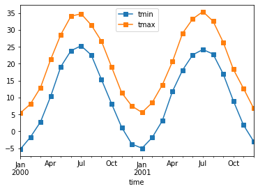
Note that MS here refers to Month-Start; M labels Month-End (the last day of the month).
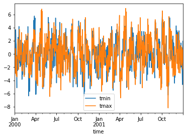
Calculate monthly anomalies
In climatology, “anomalies” refer to the difference between observations and typical weather for a particular season. Unlike observations, anomalies should not show any seasonal cycle.
[9]:
climatology = ds.groupby("time.month").mean("time")
anomalies = ds.groupby("time.month") - climatology
anomalies.mean("location").to_dataframe()[["tmin", "tmax"]].plot()
[9]:
<matplotlib.axes._subplots.AxesSubplot at 0x7f046ae37d60>
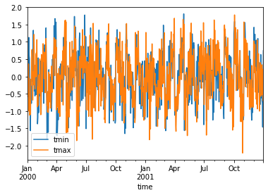
Calculate standardized monthly anomalies
You can create standardized anomalies where the difference between the observations and the climatological monthly mean is divided by the climatological standard deviation.
[10]:
climatology_mean = ds.groupby("time.month").mean("time")
climatology_std = ds.groupby("time.month").std("time")
stand_anomalies = xr.apply_ufunc(
    lambda x, m, s: (x - m) / s,
    ds.groupby("time.month"),
    climatology_mean,
    climatology_std,
)

stand_anomalies.mean("location").to_dataframe()[["tmin", "tmax"]].plot()
[10]:
<matplotlib.axes._subplots.AxesSubplot at 0x7f046ad738e0>
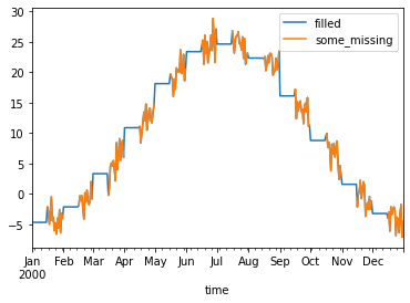
Fill missing values with climatology
The fillna method on grouped objects lets you easily fill missing values by group:
[11]:
# throw away the first half of every month
some_missing = ds.tmin.sel(time=ds["time.day"] > 15).reindex_like(ds)
filled = some_missing.groupby("time.month").fillna(climatology.tmin)
both = xr.Dataset({"some_missing": some_missing, "filled": filled})
both
[11]:
xarray.Dataset
- location: 3
- time: 731
- time(time)datetime64[ns]2000-01-01 ... 2001-12-31
array(['2000-01-01T00:00:00.000000000', '2000-01-02T00:00:00.000000000', '2000-01-03T00:00:00.000000000', ..., '2001-12-29T00:00:00.000000000', '2001-12-30T00:00:00.000000000', '2001-12-31T00:00:00.000000000'], dtype='datetime64[ns]') - location(location)object'IA' 'IN' 'IL'
array(['IA', 'IN', 'IL'], dtype=object)
- month(time)int641 1 1 1 1 1 1 ... 12 12 12 12 12 12
array([ 1,  1,  1,  1,  1,  1,  1,  1,  1,  1,  1,  1,  1,  1,  1,  1,  1,
        1,  1,  1,  1,  1,  1,  1,  1,  1,  1,  1,  1,  1,  1,  2,  2,  2,
        2,  2,  2,  2,  2,  2,  2,  2,  2,  2,  2,  2,  2,  2,  2,  2,  2,
        2,  2,  2,  2,  2,  2,  2,  2,  2,  3,  3,  3,  3,  3,  3,  3,  3,
        3,  3,  3,  3,  3,  3,  3,  3,  3,  3,  3,  3,  3,  3,  3,  3,  3,
        3,  3,  3,  3,  3,  3,  4,  4,  4,  4,  4,  4,  4,  4,  4,  4,  4,
        4,  4,  4,  4,  4,  4,  4,  4,  4,  4,  4,  4,  4,  4,  4,  4,  4,
        4,  4,  5,  5,  5,  5,  5,  5,  5,  5,  5,  5,  5,  5,  5,  5,  5,
        5,  5,  5,  5,  5,  5,  5,  5,  5,  5,  5,  5,  5,  5,  5,  5,  6,
        6,  6,  6,  6,  6,  6,  6,  6,  6,  6,  6,  6,  6,  6,  6,  6,  6,
        6,  6,  6,  6,  6,  6,  6,  6,  6,  6,  6,  6,  7,  7,  7,  7,  7,
        7,  7,  7,  7,  7,  7,  7,  7,  7,  7,  7,  7,  7,  7,  7,  7,  7,
        7,  7,  7,  7,  7,  7,  7,  7,  7,  8,  8,  8,  8,  8,  8,  8,  8,
        8,  8,  8,  8,  8,  8,  8,  8,  8,  8,  8,  8,  8,  8,  8,  8,  8,
        8,  8,  8,  8,  8,  8,  9,  9,  9,  9,  9,  9,  9,  9,  9,  9,  9,
        9,  9,  9,  9,  9,  9,  9,  9,  9,  9,  9,  9,  9,  9,  9,  9,  9,
        9,  9, 10, 10, 10, 10, 10, 10, 10, 10, 10, 10, 10, 10, 10, 10, 10,
       10, 10, 10, 10, 10, 10, 10, 10, 10, 10, 10, 10, 10, 10, 10, 10, 11,
       11, 11, 11, 11, 11, 11, 11, 11, 11, 11, 11, 11, 11, 11, 11, 11, 11,
       11, 11, 11, 11, 11, 11, 11, 11, 11, 11, 11, 11, 12, 12, 12, 12, 12,
       12, 12, 12, 12, 12, 12, 12, 12, 12, 12, 12, 12, 12, 12, 12, 12, 12,
       12, 12, 12, 12, 12, 12, 12, 12, 12,  1,  1,  1,  1,  1,  1,  1,  1,
        1,  1,  1,  1,  1,  1,  1,  1,  1,  1,  1,  1,  1,  1,  1,  1,  1,
        1,  1,  1,  1,  1,  1,  2,  2,  2,  2,  2,  2,  2,  2,  2,  2,  2,
        2,  2,  2,  2,  2,  2,  2,  2,  2,  2,  2,  2,  2,  2,  2,  2,  2,
        3,  3,  3,  3,  3,  3,  3,  3,  3,  3,  3,  3,  3,  3,  3,  3,  3,
        3,  3,  3,  3,  3,  3,  3,  3,  3,  3,  3,  3,  3,  3,  4,  4,  4,
        4,  4,  4,  4,  4,  4,  4,  4,  4,  4,  4,  4,  4,  4,  4,  4,  4,
        4,  4,  4,  4,  4,  4,  4,  4,  4,  4,  5,  5,  5,  5,  5,  5,  5,
        5,  5,  5,  5,  5,  5,  5,  5,  5,  5,  5,  5,  5,  5,  5,  5,  5,
        5,  5,  5,  5,  5,  5,  5,  6,  6,  6,  6,  6,  6,  6,  6,  6,  6,
        6,  6,  6,  6,  6,  6,  6,  6,  6,  6,  6,  6,  6,  6,  6,  6,  6,
        6,  6,  6,  7,  7,  7,  7,  7,  7,  7,  7,  7,  7,  7,  7,  7,  7,
        7,  7,  7,  7,  7,  7,  7,  7,  7,  7,  7,  7,  7,  7,  7,  7,  7,
        8,  8,  8,  8,  8,  8,  8,  8,  8,  8,  8,  8,  8,  8,  8,  8,  8,
        8,  8,  8,  8,  8,  8,  8,  8,  8,  8,  8,  8,  8,  8,  9,  9,  9,
        9,  9,  9,  9,  9,  9,  9,  9,  9,  9,  9,  9,  9,  9,  9,  9,  9,
        9,  9,  9,  9,  9,  9,  9,  9,  9,  9, 10, 10, 10, 10, 10, 10, 10,
       10, 10, 10, 10, 10, 10, 10, 10, 10, 10, 10, 10, 10, 10, 10, 10, 10,
       10, 10, 10, 10, 10, 10, 10, 11, 11, 11, 11, 11, 11, 11, 11, 11, 11,
       11, 11, 11, 11, 11, 11, 11, 11, 11, 11, 11, 11, 11, 11, 11, 11, 11,
       11, 11, 11, 12, 12, 12, 12, 12, 12, 12, 12, 12, 12, 12, 12, 12, 12,
       12, 12, 12, 12, 12, 12, 12, 12, 12, 12, 12, 12, 12, 12, 12, 12, 12])
- some_missing(time, location)float64nan nan nan ... 2.063 -1.346 -4.544
array([[ nan, nan, nan], [ nan, nan, nan], [ nan, nan, nan], ..., [ -5.34723825, -13.37459826, -4.93221199], [ -2.67283594, -5.18072141, -4.11567869], [ 2.06327582, -1.34576404, -4.54392729]]) - filled(time, location)float64-5.163 -4.216 ... -1.346 -4.544
array([[ -5.16274935,  -4.21616663,  -4.68137385],
       [ -5.16274935,  -4.21616663,  -4.68137385],
       [ -5.16274935,  -4.21616663,  -4.68137385],
       ...,
       [ -5.34723825, -13.37459826,  -4.93221199],
       [ -2.67283594,  -5.18072141,  -4.11567869],
       [  2.06327582,  -1.34576404,  -4.54392729]])
[12]:
df = both.sel(time="2000").mean("location").reset_coords(drop=True).to_dataframe()
df.head()
/home/docs/checkouts/readthedocs.org/user_builds/xray/checkouts/v0.15.1/xarray/core/nanops.py:142: RuntimeWarning: Mean of empty slice
  return np.nanmean(a, axis=axis, dtype=dtype)
[12]:
| some_missing | filled | |
|---|---|---|
| time | ||
| 2000-01-01 | NaN | -4.686763 |
| 2000-01-02 | NaN | -4.686763 |
| 2000-01-03 | NaN | -4.686763 |
| 2000-01-04 | NaN | -4.686763 |
| 2000-01-05 | NaN | -4.686763 |
[13]:
df[["filled", "some_missing"]].plot()
[13]:
<matplotlib.axes._subplots.AxesSubplot at 0x7f046ac83700>