You can run this notebook in a live session or view it on Github.

ROMS Ocean Model Example

The Regional Ocean Modeling System (ROMS) is an open source hydrodynamic model that is used for simulating currents and water properties in coastal and estuarine regions. ROMS is one of a few standard ocean models, and it has an active user community.

ROMS uses a regular C-Grid in the horizontal, similar to other structured grid ocean and atmospheric models, and a stretched vertical coordinate (see the ROMS documentation for more details). Both of these require special treatment when using xarray to analyze ROMS ocean model output. This example notebook shows how to create a lazily evaluated vertical coordinate, and make some basic plots. The xgcm package is required to do analysis that is aware of the horizontal C-Grid.

import numpy as np
import cartopy.crs as ccrs
import cartopy.feature as cfeature
import matplotlib.pyplot as plt
%matplotlib inline

import xarray as xr

Load a sample ROMS file. This is a subset of a full model available at

http://barataria.tamu.edu/thredds/catalog.html?dataset=txla_hindcast_agg

The subsetting was done using the following command on one of the output files:

#open dataset
ds = xr.open_dataset('/d2/shared/TXLA_ROMS/output_20yr_obc/2001/ocean_his_0015.nc')

# Turn on chunking to activate dask and parallelize read/write.
ds = ds.chunk({'ocean_time': 1})

# Pick out some of the variables that will be included as coordinates
ds = ds.set_coords(['Cs_r', 'Cs_w', 'hc', 'h', 'Vtransform'])

# Select a a subset of variables. Salt will be visualized, zeta is used to
# calculate the vertical coordinate
variables = ['salt', 'zeta']
ds[variables].isel(ocean_time=slice(47, None, 7*24),
                   xi_rho=slice(300, None)).to_netcdf('ROMS_example.nc', mode='w')

So, the ROMS_example.nc file contains a subset of the grid, one 3D variable, and two time steps.

Load in ROMS dataset as an xarray object

# load in the file
ds = xr.tutorial.open_dataset('ROMS_example.nc', chunks={'ocean_time': 1})

# This is a way to turn on chunking and lazy evaluation. Opening with mfdataset, or
# setting the chunking in the open_dataset would also achive this.
ds

xarray.Dataset

• Dimensions:
  • eta_rho: 191
  • ocean_time: 2
  • s_rho: 30
  • xi_rho: 371
• Coordinates: (8)
  • Cs_r
    (s_rho)
    float64
    dask.array<chunksize=(30,), meta=np.ndarray>

    long_name :

    S-coordinate stretching curves at RHO-points

    valid_min :

    -1.0

    valid_max :

    0.0

    field :

    Cs_r, scalar

    
    
    
    
      
    
        
     
     Array 
     Chunk 
      
      
    
        
     Bytes 
     240 B 
     
     240 B 
        
     Shape 
     (30,) 
     
     (30,) 
        
     Count 
     2 Tasks 
     1 Chunks 
        
     Type 
     float64 
     numpy.ndarray 
      
    
    
    
    
    
    
    

  • lon_rho
    (eta_rho, xi_rho)
    float64
    dask.array<chunksize=(191, 371), meta=np.ndarray>

    long_name :

    longitude of RHO-points

    units :

    degree_east

    standard_name :

    longitude

    field :

    lon_rho, scalar

    
    
    
    
      
    
        
     
     Array 
     Chunk 
      
      
    
        
     Bytes 
     566.89 kB 
     
     566.89 kB 
        
     Shape 
     (191, 371) 
     
     (191, 371) 
        
     Count 
     2 Tasks 
     1 Chunks 
        
     Type 
     float64 
     numpy.ndarray 
      
    
    
    
    
    
    
    

  • hc
    ()
    float64
    ...

    long_name :

    S-coordinate parameter, critical depth

    units :

    meter

    array(20.)

  • h
    (eta_rho, xi_rho)
    float64
    dask.array<chunksize=(191, 371), meta=np.ndarray>

    long_name :

    bathymetry at RHO-points

    units :

    meter

    field :

    bath, scalar

    
    
    
    
      
    
        
     
     Array 
     Chunk 
      
      
    
        
     Bytes 
     566.89 kB 
     
     566.89 kB 
        
     Shape 
     (191, 371) 
     
     (191, 371) 
        
     Count 
     2 Tasks 
     1 Chunks 
        
     Type 
     float64 
     numpy.ndarray 
      
    
    
    
    
    
    
    

  • lat_rho
    (eta_rho, xi_rho)
    float64
    dask.array<chunksize=(191, 371), meta=np.ndarray>

    long_name :

    latitude of RHO-points

    units :

    degree_north

    standard_name :

    latitude

    field :

    lat_rho, scalar

    
    
    
    
      
    
        
     
     Array 
     Chunk 
      
      
    
        
     Bytes 
     566.89 kB 
     
     566.89 kB 
        
     Shape 
     (191, 371) 
     
     (191, 371) 
        
     Count 
     2 Tasks 
     1 Chunks 
        
     Type 
     float64 
     numpy.ndarray 
      
    
    
    
    
    
    
    

  • Vtransform
    ()
    int32
    ...

    long_name :

    vertical terrain-following transformation equation

    array(2, dtype=int32)

  • ocean_time
    (ocean_time)
    datetime64[ns]
    2001-08-01 2001-08-08

    long_name :

    time since initialization

    field :

    time, scalar, series

    array(['2001-08-01T00:00:00.000000000', '2001-08-08T00:00:00.000000000'],
          dtype='datetime64[ns]')

  • s_rho
    (s_rho)
    float64
    -0.9833 -0.95 ... -0.05 -0.01667

    long_name :

    S-coordinate at RHO-points

    valid_min :

    -1.0

    valid_max :

    0.0

    positive :

    up

    standard_name :

    ocean_s_coordinate_g2

    formula_terms :

    s: s_rho C: Cs_r eta: zeta depth: h depth_c: hc

    field :

    s_rho, scalar

    array([-0.983333, -0.95    , -0.916667, -0.883333, -0.85    , -0.816667,
           -0.783333, -0.75    , -0.716667, -0.683333, -0.65    , -0.616667,
           -0.583333, -0.55    , -0.516667, -0.483333, -0.45    , -0.416667,
           -0.383333, -0.35    , -0.316667, -0.283333, -0.25    , -0.216667,
           -0.183333, -0.15    , -0.116667, -0.083333, -0.05    , -0.016667])

• Data variables: (2)
  • salt
    (ocean_time, s_rho, eta_rho, xi_rho)
    float32
    dask.array<chunksize=(1, 30, 191, 371), meta=np.ndarray>

    long_name :

    salinity

    time :

    ocean_time

    field :

    salinity, scalar, series

    
    
    
    
      
    
        
     
     Array 
     Chunk 
      
      
    
        
     Bytes 
     17.01 MB 
     
     8.50 MB 
        
     Shape 
     (2, 30, 191, 371) 
     
     (1, 30, 191, 371) 
        
     Count 
     3 Tasks 
     2 Chunks 
        
     Type 
     float32 
     numpy.ndarray 
      
    
    
    
    
    
    
    

  • zeta
    (ocean_time, eta_rho, xi_rho)
    float32
    dask.array<chunksize=(1, 191, 371), meta=np.ndarray>

    long_name :

    free-surface

    units :

    meter

    time :

    ocean_time

    field :

    free-surface, scalar, series

    
    
    
    
      
    
        
     
     Array 
     Chunk 
      
      
    
        
     Bytes 
     566.89 kB 
     
     283.44 kB 
        
     Shape 
     (2, 191, 371) 
     
     (1, 191, 371) 
        
     Count 
     3 Tasks 
     2 Chunks 
        
     Type 
     float32 
     numpy.ndarray 
      
    
    
    
    
    
    
    

• Attributes: (34)

  file :

  ../output_20yr_obc/2001/ocean_his_0015.nc

  format :

  netCDF-4/HDF5 file

  Conventions :

  CF-1.4

  type :

  ROMS/TOMS history file

  title :

  TXLA ROMS hindcast run with dyes and oxygen

  rst_file :

  ../output_20yr_obc/2001/ocean_rst.nc

  his_base :

  ../output_20yr_obc/2001/ocean_his

  avg_base :

  ../output_20yr_obc/2001/ocean_avg

  dia_base :

  ../output_20yr_obc/2001/ocean_dia

  sta_file :

  ocean_sta.nc

  grd_file :

  ../inputs/grd/txla2_grd_v4_test_lcut_hglo_wtype.nc

  ini_file :

  ../output_20yr_obc/2000/ocean_rst.nc

  frc_file_01 :

  ../inputs/2001/txla_bulk_ERAI_2001.nc

  frc_file_02 :

  ../inputs/2001/txla_flx_ICOADS_AVHRR_SST_2001.nc, ../inputs/2002/txla_flx_ICOADS_AVHRR_SST_2002.nc

  bry_file_01 :

  ../inputs/2001/txla2_bry_2001_glo_ReAna_v4_o2woa.nc, ../inputs/2002/txla2_bry_2002_glo_ReAna_v4_o2woa.nc

  clm_file_01 :

  ../inputs/2001/txla2_clm_2001_01_glo_ReAna_v4_o2woa.nc, ../inputs/2001/txla2_clm_2001_02_glo_ReAna_v4_o2woa.nc, ../inputs/2001/txla2_clm_2001_03_glo_ReAna_v4_o2woa.nc, ../inputs/2001/txla2_clm_2001_04_glo_ReAna_v4_o2woa.nc, ../inputs/2001/txla2_clm_2001_05_glo_ReAna_v4_o2woa.nc, ../inputs/2001/txla2_clm_2001_06_glo_ReAna_v4_o2woa.nc, ../inputs/2001/txla2_clm_2001_07_glo_ReAna_v4_o2woa.nc, ../inputs/2001/txla2_clm_2001_08_glo_ReAna_v4_o2woa.nc, ../inputs/2001/txla2_clm_2001_09_glo_ReAna_v4_o2woa.nc, ../inputs/2001/txla2_clm_2001_10_glo_ReAna_v4_o2woa.nc, ../inputs/2001/txla2_clm_2001_11_glo_ReAna_v4_o2woa.nc, ../inputs/2001/txla2_clm_2001_12_glo_ReAna_v4_o2woa.nc, ../inputs/2002/txla2_clm_2002_01_glo_ReAna_v4_o2woa.nc

  script_file :

  spos_file :

  /scratch/user/d.kobashi/inputs/stations.in

  NLM_LBC :

  EDGE: WEST SOUTH EAST NORTH zeta: Che Che Che Clo ubar: Shc Shc Shc Clo vbar: Shc Shc Shc Clo u: Rad Rad Rad Clo v: Rad Rad Rad Clo temp: Rad Rad Rad Clo salt: Rad Rad Rad Clo dye_01: Gra Gra Gra Clo dye_02: Rad Rad Rad Clo dye_03: Rad Rad Rad Clo dye_04: Rad Rad Rad Clo tke: Gra Gra Gra Clo

  svn_url :

  https:://myroms.org/svn/src

  svn_rev :

  code_dir :

  /scratch/user/d.kobashi/source_code/COAWST/COAWST.r960-dev

  header_dir :

  /home/d.kobashi/TXLA_ROMS_reana/work_20yr_obc

  header_file :

  txla2.h

  os :

  Linux

  cpu :

  x86_64

  compiler_system :

  ifort

  compiler_command :

  /software/easybuild/software/impi/5.0.1.035-iccifort-2015.0.090/bin64/mpiifort

  compiler_flags :

  -heap-arrays -fp-model fast -mt_mpi -ip -O3 -msse2 -free

  tiling :

  010x012

  history :

  Tue Jul 24 11:04:43 2018: /opt/nco/ncks -D 4 -t 8 /copano/d1/shared/TXLA_ROMS/output_20yr_obc/2001/ocean_his_0015.nc --cnk_dmn ocean_time,4 --cnk_dmn eta_rho,8 --cnk_dmn eta_u,8 --cnk_dmn eta_v,8 --cnk_dmn eta_psi,8 --cnk_dmn xi_rho,16 --cnk_dmn xi_u,16 --cnk_dmn xi_v,16 --cnk_dmn xi_psi,16 --cnk_dmn s_rho,2 --cnk_dmn s_w,2 --output /copano/d2/shared/TXLA_ROMS/output_20yr_obc/2001/ocean_his_0015.nc ROMS/TOMS, Version 3.7, Monday - July 18, 2016 - 10:38:26 PM

  ana_file :

  /home/d.kobashi/TXLA_ROMS_reana/Functionals/ana_btflux.h, /home/d.kobashi/TXLA_ROMS_reana/Functionals/ana_sponge.h, /home/d.kobashi/TXLA_ROMS_reana/Functionals/ana_nudgcoef.h, /home/d.kobashi/TXLA_ROMS_reana/Functionals/ana_stflux.h

  CPP_options :

  TXLA2, ANA_BPFLUX, ANA_BSFLUX, ANA_BTFLUX, ANA_NUDGCOEF, ANA_SPFLUX, ANA_SPONGE, ASSUMED_SHAPE, AVERAGES, BULK_FLUXES, CURVGRID, DEFLATE, DIAGNOSTICS_TS, DIAGNOSTICS_UV, DIFF_GRID, DJ_GRADPS, DOUBLE_PRECISION, EMINUSP, GLS_MIXING, HDF5, KANTHA_CLAYSON, LONGWAVE, MASKING, MIX_GEO_TS, MIX_S_UV, MPI, NONLINEAR, NONLIN_EOS, N2S2_HORAVG, POWER_LAW, PROFILE, QCORRECTION, K_GSCHEME, RADIATION_2D, !RST_SINGLE, SALINITY, SOLAR_SOURCE, SOLVE3D, SPLINES, SPHERICAL, STATIONS, T_PASSIVE, TS_MPDATA, TS_DIF2, UV_ADV, UV_COR, UV_U3HADVECTION, UV_C4VADVECTION, UV_LOGDRAG, UV_VIS2, VAR_RHO_2D, VISC_GRID, WTYPE_GRID

  NCO :

  netCDF Operators version 4.7.6-alpha04 (Homepage = http://nco.sf.net, Code = http://github.com/nco/nco)

Add a lazilly calculated vertical coordinates

Write equations to calculate the vertical coordinate. These will be only evaluated when data is requested. Information about the ROMS vertical coordinate can be found (here)[https://www.myroms.org/wiki/Vertical_S-coordinate]

In short, for Vtransform==2 as used in this example,

\(Z_0 = (h_c \, S + h \,C) / (h_c + h)\)

\(z = Z_0 (\zeta + h) + \zeta\)

where the variables are defined as in the link above.

if ds.Vtransform == 1:
    Zo_rho = ds.hc * (ds.s_rho - ds.Cs_r) + ds.Cs_r * ds.h
    z_rho = Zo_rho + ds.zeta * (1 + Zo_rho/ds.h)
elif ds.Vtransform == 2:
    Zo_rho = (ds.hc * ds.s_rho + ds.Cs_r * ds.h) / (ds.hc + ds.h)
    z_rho = ds.zeta + (ds.zeta + ds.h) * Zo_rho

ds.coords['z_rho'] = z_rho.transpose()   # needing transpose seems to be an xarray bug
ds.salt

<ipython-input-3-8742ef454e3d>:8: FutureWarning: This DataArray contains multi-dimensional coordinates. In the future, these coordinates will be transposed as well unless you specify transpose_coords=False.
  ds.coords['z_rho'] = z_rho.transpose()   # needing transpose seems to be an xarray bug

xarray.DataArray

'salt'

• ocean_time: 2
• s_rho: 30
• eta_rho: 191
• xi_rho: 371

• dask.array<chunksize=(1, 30, 191, 371), meta=np.ndarray>

  
  
  
  
    
  
      
   
   Array 
   Chunk 
    
    
  
      
   Bytes 
   17.01 MB 
   
   8.50 MB 
      
   Shape 
   (2, 30, 191, 371) 
   
   (1, 30, 191, 371) 
      
   Count 
   3 Tasks 
   2 Chunks 
      
   Type 
   float32 
   numpy.ndarray 
    
  
  
  
  
  
  
  

• Coordinates: (9)
  • Cs_r
    (s_rho)
    float64
    dask.array<chunksize=(30,), meta=np.ndarray>

    long_name :

    S-coordinate stretching curves at RHO-points

    valid_min :

    -1.0

    valid_max :

    0.0

    field :

    Cs_r, scalar

    
    
    
    
      
    
        
     
     Array 
     Chunk 
      
      
    
        
     Bytes 
     240 B 
     
     240 B 
        
     Shape 
     (30,) 
     
     (30,) 
        
     Count 
     2 Tasks 
     1 Chunks 
        
     Type 
     float64 
     numpy.ndarray 
      
    
    
    
    
    
    
    

  • lon_rho
    (eta_rho, xi_rho)
    float64
    dask.array<chunksize=(191, 371), meta=np.ndarray>

    long_name :

    longitude of RHO-points

    units :

    degree_east

    standard_name :

    longitude

    field :

    lon_rho, scalar

    
    
    
    
      
    
        
     
     Array 
     Chunk 
      
      
    
        
     Bytes 
     566.89 kB 
     
     566.89 kB 
        
     Shape 
     (191, 371) 
     
     (191, 371) 
        
     Count 
     2 Tasks 
     1 Chunks 
        
     Type 
     float64 
     numpy.ndarray 
      
    
    
    
    
    
    
    

  • hc
    ()
    float64
    20.0

    long_name :

    S-coordinate parameter, critical depth

    units :

    meter

    array(20.)

  • h
    (eta_rho, xi_rho)
    float64
    dask.array<chunksize=(191, 371), meta=np.ndarray>

    long_name :

    bathymetry at RHO-points

    units :

    meter

    field :

    bath, scalar

    
    
    
    
      
    
        
     
     Array 
     Chunk 
      
      
    
        
     Bytes 
     566.89 kB 
     
     566.89 kB 
        
     Shape 
     (191, 371) 
     
     (191, 371) 
        
     Count 
     2 Tasks 
     1 Chunks 
        
     Type 
     float64 
     numpy.ndarray 
      
    
    
    
    
    
    
    

  • lat_rho
    (eta_rho, xi_rho)
    float64
    dask.array<chunksize=(191, 371), meta=np.ndarray>

    long_name :

    latitude of RHO-points

    units :

    degree_north

    standard_name :

    latitude

    field :

    lat_rho, scalar

    
    
    
    
      
    
        
     
     Array 
     Chunk 
      
      
    
        
     Bytes 
     566.89 kB 
     
     566.89 kB 
        
     Shape 
     (191, 371) 
     
     (191, 371) 
        
     Count 
     2 Tasks 
     1 Chunks 
        
     Type 
     float64 
     numpy.ndarray 
      
    
    
    
    
    
    
    

  • Vtransform
    ()
    int32
    2

    long_name :

    vertical terrain-following transformation equation

    array(2, dtype=int32)

  • ocean_time
    (ocean_time)
    datetime64[ns]
    2001-08-01 2001-08-08

    long_name :

    time since initialization

    field :

    time, scalar, series

    array(['2001-08-01T00:00:00.000000000', '2001-08-08T00:00:00.000000000'],
          dtype='datetime64[ns]')

  • s_rho
    (s_rho)
    float64
    -0.9833 -0.95 ... -0.05 -0.01667

    long_name :

    S-coordinate at RHO-points

    valid_min :

    -1.0

    valid_max :

    0.0

    positive :

    up

    standard_name :

    ocean_s_coordinate_g2

    formula_terms :

    s: s_rho C: Cs_r eta: zeta depth: h depth_c: hc

    field :

    s_rho, scalar

    array([-0.983333, -0.95    , -0.916667, -0.883333, -0.85    , -0.816667,
           -0.783333, -0.75    , -0.716667, -0.683333, -0.65    , -0.616667,
           -0.583333, -0.55    , -0.516667, -0.483333, -0.45    , -0.416667,
           -0.383333, -0.35    , -0.316667, -0.283333, -0.25    , -0.216667,
           -0.183333, -0.15    , -0.116667, -0.083333, -0.05    , -0.016667])

  • z_rho
    (s_rho, xi_rho, eta_rho, ocean_time)
    float64
    dask.array<chunksize=(30, 371, 191, 1), meta=np.ndarray>

    
    
    
    
      
    
        
     
     Array 
     Chunk 
      
      
    
        
     Bytes 
     34.01 MB 
     
     17.01 MB 
        
     Shape 
     (30, 371, 191, 2) 
     
     (30, 371, 191, 1) 
        
     Count 
     35 Tasks 
     2 Chunks 
        
     Type 
     float64 
     numpy.ndarray 
      
    
    
    
    
    
    
    

• Attributes: (3)

  long_name :

  salinity

  time :

  ocean_time

  field :

  salinity, scalar, series

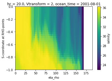
A naive vertical slice

Create a slice using the s-coordinate as the vertical dimension is typically not very informative.

ds.salt.isel(xi_rho=50, ocean_time=0).plot()

<matplotlib.collections.QuadMesh at 0x7f1ce22a2a30>

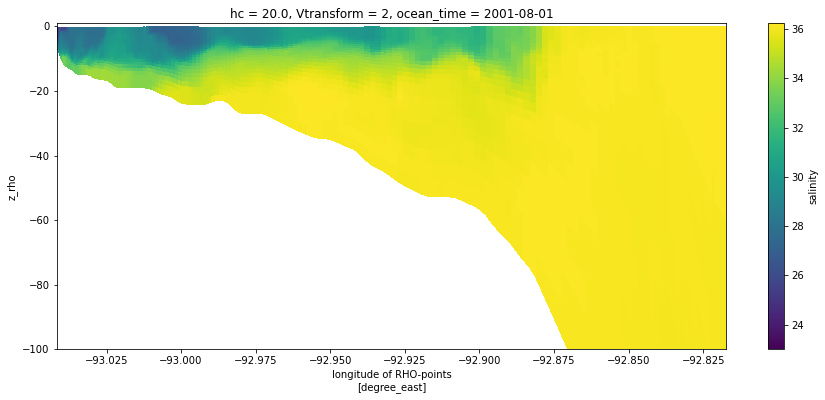
We can feed coordinate information to the plot method to give a more informative cross-section that uses the depths. Note that we did not need to slice the depth or longitude information separately, this was done automatically as the variable was sliced.

section = ds.salt.isel(xi_rho=50, eta_rho=slice(0, 167), ocean_time=0)
section.plot(x='lon_rho', y='z_rho', figsize=(15, 6), clim=(25, 35))
plt.ylim([-100, 1]);

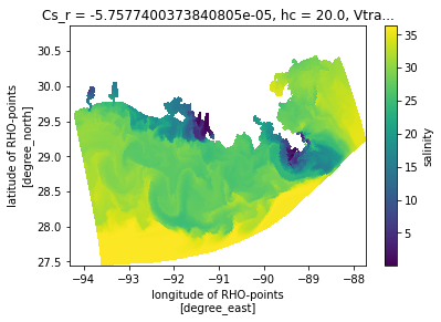
A plan view

Now make a naive plan view, without any projection information, just using lon/lat as x/y. This looks OK, but will appear compressed because lon and lat do not have an aspect constrained by the projection.

ds.salt.isel(s_rho=-1, ocean_time=0).plot(x='lon_rho', y='lat_rho')

<matplotlib.collections.QuadMesh at 0x7f1ce20a4fd0>

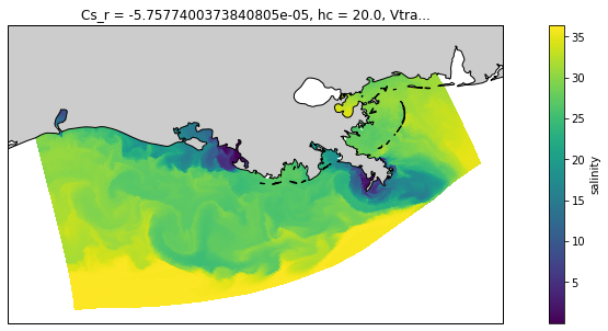
And let’s use a projection to make it nicer, and add a coast.

proj = ccrs.LambertConformal(central_longitude=-92, central_latitude=29)
fig = plt.figure(figsize=(15, 5))
ax = plt.axes(projection=proj)
ds.salt.isel(s_rho=-1, ocean_time=0).plot(x='lon_rho', y='lat_rho',
                                          transform=ccrs.PlateCarree())

coast_10m = cfeature.NaturalEarthFeature('physical', 'land', '10m',
                                        edgecolor='k', facecolor='0.8')
ax.add_feature(coast_10m)

<cartopy.mpl.feature_artist.FeatureArtist at 0x7f1ce21bc8e0>

/home/docs/checkouts/readthedocs.org/user_builds/xray/conda/v0.15.1/lib/python3.8/site-packages/cartopy/io/__init__.py:260: DownloadWarning: Downloading: http://naciscdn.org/naturalearth/10m/physical/ne_10m_land.zip
  warnings.warn('Downloading: {}'.format(url), DownloadWarning)