Serialization and IO
xarray supports direct serialization and IO to several file formats, from simple Pickle files to the more flexible netCDF format.
Pickle
The simplest way to serialize an xarray object is to use Python’s built-in pickle module:
In [1]: import pickle

In [2]: ds = xr.Dataset({'foo': (('x', 'y'), np.random.rand(4, 5))},
   ...:                 coords={'x': [10, 20, 30, 40],
   ...:                         'y': pd.date_range('2000-01-01', periods=5),
   ...:                         'z': ('x', list('abcd'))})
   ...:

# use the highest protocol (-1) because it is way faster than the default
# text based pickle format
In [3]: pkl = pickle.dumps(ds, protocol=-1)

In [4]: pickle.loads(pkl)
Out[4]:
<xarray.Dataset>
Dimensions:  (x: 4, y: 5)
Coordinates:
  * y        (y) datetime64[ns] 2000-01-01 2000-01-02 2000-01-03 2000-01-04 ...
    z        (x) <U1 'a' 'b' 'c' 'd'
  * x        (x) int64 10 20 30 40
Data variables:
    foo      (x, y) float64 0.127 0.9667 0.2605 0.8972 0.3767 0.3362 0.4514 ...
Pickle support is important because it doesn’t require any external libraries
and lets you use xarray objects with Python modules like
multiprocessing. However, there are two important caveats:
- To simplify serialization, xarray’s support for pickle currently loads all array values into memory before dumping an object. This means it is not suitable for serializing datasets too big to load into memory (e.g., from netCDF or OPeNDAP).
- Pickle will only work as long as the internal data structure of xarray objects remains unchanged. Because the internal design of xarray is still being refined, we make no guarantees (at this point) that objects pickled with this version of xarray will work in future versions.
Dictionary
We can convert a Dataset (or a DataArray) to a dict using
to_dict():
In [5]: d = ds.to_dict()

In [6]: d
Out[6]:
{'attrs': {},
 'coords': {'x': {'attrs': {}, 'data': [10, 20, 30, 40], 'dims': ('x',)},
  'y': {'attrs': {},
   'data': [datetime.datetime(2000, 1, 1, 0, 0),
    datetime.datetime(2000, 1, 2, 0, 0),
    datetime.datetime(2000, 1, 3, 0, 0),
    datetime.datetime(2000, 1, 4, 0, 0),
    datetime.datetime(2000, 1, 5, 0, 0)],
   'dims': ('y',)},
  'z': {'attrs': {}, 'data': ['a', 'b', 'c', 'd'], 'dims': ('x',)}},
 'data_vars': {'foo': {'attrs': {},
   'data': [[0.12696983303810094,
     0.966717838482003,
     0.26047600586578334,
     0.8972365243645735,
     0.37674971618967135],
    [0.33622174433445307,
     0.45137647047539964,
     0.8402550832613813,
     0.12310214428849964,
     0.5430262020470384],
    [0.37301222522143085,
     0.4479968246859435,
     0.12944067971751294,
     0.8598787065799693,
     0.8203883631195572],
    [0.35205353914802473,
     0.2288873043216132,
     0.7767837505077176,
     0.5947835894851238,
     0.1375535565632705]],
   'dims': ('x', 'y')}},
 'dims': {'x': 4, 'y': 5}}
We can create a new xarray object from a dict using
from_dict():
In [7]: ds_dict = xr.Dataset.from_dict(d)

In [8]: ds_dict
Out[8]:
<xarray.Dataset>
Dimensions:  (x: 4, y: 5)
Coordinates:
  * y        (y) datetime64[ns] 2000-01-01 2000-01-02 2000-01-03 2000-01-04 ...
    z        (x) <U1 'a' 'b' 'c' 'd'
  * x        (x) int64 10 20 30 40
Data variables:
    foo      (x, y) float64 0.127 0.9667 0.2605 0.8972 0.3767 0.3362 0.4514 ...
Dictionary support allows for flexible use of xarray objects. It doesn’t require external libraries and dicts can easily be pickled, or converted to json, or geojson. All the values are converted to lists, so dicts might be quite large.
netCDF
The recommended way to store xarray data structures is netCDF, which
is a binary file format for self-described datasets that originated
in the geosciences. xarray is based on the netCDF data model, so netCDF files
on disk directly correspond to Dataset objects.
NetCDF is supported on almost all platforms, and parsers exist for the vast majority of scientific programming languages. Recent versions of netCDF are based on the even more widely used HDF5 file-format.
Tip
If you aren’t familiar with this data format, the netCDF FAQ is a good place to start.
Reading and writing netCDF files with xarray requires scipy or the netCDF4-Python library to be installed (the later is required to read/write netCDF V4 files and use the compression options described below).
We can save a Dataset to disk using the
Dataset.to_netcdf method:
In [9]: ds.to_netcdf('saved_on_disk.nc')
By default, the file is saved as netCDF4 (assuming netCDF4-Python is
installed). You can control the format and engine used to write the file with
the format and engine arguments.
We can load netCDF files to create a new Dataset using
open_dataset():
In [10]: ds_disk = xr.open_dataset('saved_on_disk.nc')

In [11]: ds_disk
Out[11]:
<xarray.Dataset>
Dimensions:  (x: 4, y: 5)
Coordinates:
  * y        (y) datetime64[ns] 2000-01-01 2000-01-02 2000-01-03 2000-01-04 ...
    z        (x) object 'a' 'b' 'c' 'd'
  * x        (x) int64 10 20 30 40
Data variables:
    foo      (x, y) float64 0.127 0.9667 0.2605 0.8972 0.3767 0.3362 0.4514 ...
Similarly, a DataArray can be saved to disk using the
DataArray.to_netcdf method, and loaded
from disk using the open_dataarray() function. As netCDF files
correspond to Dataset objects, these functions internally
convert the DataArray to a Dataset before saving, and then convert back
when loading, ensuring that the DataArray that is loaded is always exactly
the same as the one that was saved.
A dataset can also be loaded or written to a specific group within a netCDF
file. To load from a group, pass a group keyword argument to the
open_dataset function. The group can be specified as a path-like
string, e.g., to access subgroup ‘bar’ within group ‘foo’ pass
‘/foo/bar’ as the group argument. When writing multiple groups in one file,
pass mode='a' to to_netcdf to ensure that each call does not delete the
file.
Data is always loaded lazily from netCDF files. You can manipulate, slice and subset Dataset and DataArray objects, and no array values are loaded into memory until you try to perform some sort of actual computation. For an example of how these lazy arrays work, see the OPeNDAP section below.
It is important to note that when you modify values of a Dataset, even one linked to files on disk, only the in-memory copy you are manipulating in xarray is modified: the original file on disk is never touched.
Tip
xarray’s lazy loading of remote or on-disk datasets is often but not always
desirable. Before performing computationally intense operations, it is
often a good idea to load a Dataset (or DataArray) entirely into memory by
invoking the load() method.
Datasets have a close() method to close the associated
netCDF file. However, it’s often cleaner to use a with statement:
# this automatically closes the dataset after use
In [12]: with xr.open_dataset('saved_on_disk.nc') as ds:
   ....:     print(ds.keys())
   ....:
KeysView(<xarray.Dataset>
Dimensions:  (x: 4, y: 5)
Coordinates:
  * y        (y) datetime64[ns] 2000-01-01 2000-01-02 2000-01-03 2000-01-04 ...
    z        (x) object 'a' 'b' 'c' 'd'
  * x        (x) int64 10 20 30 40
Data variables:
    foo      (x, y) float64 0.127 0.9667 0.2605 0.8972 0.3767 0.3362 0.4514 ...)
Although xarray provides reasonable support for incremental reads of files on disk, it does not support incremental writes, which can be a useful strategy for dealing with datasets too big to fit into memory. Instead, xarray integrates with dask.array (see Out of core computation with dask), which provides a fully featured engine for streaming computation.
Reading encoded data
NetCDF files follow some conventions for encoding datetime arrays (as numbers
with a “units” attribute) and for packing and unpacking data (as
described by the “scale_factor” and “add_offset” attributes). If the argument
decode_cf=True (default) is given to open_dataset, xarray will attempt
to automatically decode the values in the netCDF objects according to
CF conventions. Sometimes this will fail, for example, if a variable
has an invalid “units” or “calendar” attribute. For these cases, you can
turn this decoding off manually.
You can view this encoding information (among others) in the
DataArray.encoding attribute:
In [13]: ds_disk['y'].encoding
Out[13]:
{'calendar': u'proleptic_gregorian',
 'chunksizes': None,
 'complevel': 0,
 'contiguous': True,
 'dtype': dtype('float64'),
 'fletcher32': False,
 'least_significant_digit': None,
 'shuffle': False,
 'source': 'saved_on_disk.nc',
 'units': u'days since 2000-01-01 00:00:00',
 'zlib': False}
Note that all operations that manipulate variables other than indexing will remove encoding information.
Writing encoded data
Conversely, you can customize how xarray writes netCDF files on disk by
providing explicit encodings for each dataset variable. The encoding
argument takes a dictionary with variable names as keys and variable specific
encodings as values. These encodings are saved as attributes on the netCDF
variables on disk, which allows xarray to faithfully read encoded data back into
memory.
It is important to note that using encodings is entirely optional: if you do not
supply any of these encoding options, xarray will write data to disk using a
default encoding, or the options in the encoding attribute, if set.
This works perfectly fine in most cases, but encoding can be useful for
additional control, especially for enabling compression.
In the file on disk, these encodings as saved as attributes on each variable, which allow xarray and other CF-compliant tools for working with netCDF files to correctly read the data.
Scaling and type conversions
These encoding options work on any version of the netCDF file format:
dtype: Any valid NumPy dtype or string convertable to a dtype, e.g.,'int16'or'float32'. This controls the type of the data written on disk._FillValue: Values ofNaNin xarray variables are remapped to this value when saved on disk. This is important when converting floating point with missing values to integers on disk, becauseNaNis not a valid value for integer dtypes. As a default, variables with float types are attributed a_FillValueofNaNin the output file.scale_factorandadd_offset: Used to convert from encoded data on disk to to the decoded data in memory, according to the formuladecoded = scale_factor * encoded + add_offset.
These parameters can be fruitfully combined to compress discretized data on disk. For
example, to save the variable foo with a precision of 0.1 in 16-bit integers while
converting NaN to -9999, we would use
encoding={'foo': {'dtype': 'int16', 'scale_factor': 0.1, '_FillValue': -9999}}.
Compression and decompression with such discretization is extremely fast.
Chunk based compression
zlib, complevel, fletcher32, continguous and chunksizes
can be used for enabling netCDF4/HDF5’s chunk based compression, as described
in the documentation for createVariable for netCDF4-Python. This only works
for netCDF4 files and thus requires using format='netCDF4' and either
engine='netcdf4' or engine='h5netcdf'.
Chunk based gzip compression can yield impressive space savings, especially for sparse data, but it comes with significant performance overhead. HDF5 libraries can only read complete chunks back into memory, and maximum decompression speed is in the range of 50-100 MB/s. Worse, HDF5’s compression and decompression currently cannot be parallelized with dask. For these reasons, we recommend trying discretization based compression (described above) first.
Time units
The units and calendar attributes control how xarray serializes datetime64 and
timedelta64 arrays to datasets on disk as numeric values. The units encoding
should be a string like 'days since 1900-01-01' for datetime64 data or a string
like 'days' for timedelta64 data. calendar should be one of the calendar types
supported by netCDF4-python: ‘standard’, ‘gregorian’, ‘proleptic_gregorian’ ‘noleap’,
‘365_day’, ‘360_day’, ‘julian’, ‘all_leap’, ‘366_day’.
By default, xarray uses the ‘proleptic_gregorian’ calendar and units of the smallest time difference between values, with a reference time of the first time value.
OPeNDAP
xarray includes support for OPeNDAP (via the netCDF4 library or Pydap), which lets us access large datasets over HTTP.
For example, we can open a connection to GBs of weather data produced by the PRISM project, and hosted by IRI at Columbia:
In [14]: remote_data = xr.open_dataset(
   ....:     'http://iridl.ldeo.columbia.edu/SOURCES/.OSU/.PRISM/.monthly/dods',
   ....:     decode_times=False)
   ....:

In [15]: remote_data
Out[15]:
<xarray.Dataset>
Dimensions:  (T: 1422, X: 1405, Y: 621)
Coordinates:
  * X        (X) float32 -125.0 -124.958 -124.917 -124.875 -124.833 -124.792 -124.75 ...
  * T        (T) float32 -779.5 -778.5 -777.5 -776.5 -775.5 -774.5 -773.5 -772.5 -771.5 ...
  * Y        (Y) float32 49.9167 49.875 49.8333 49.7917 49.75 49.7083 49.6667 49.625 ...
Data variables:
    ppt      (T, Y, X) float64 ...
    tdmean   (T, Y, X) float64 ...
    tmax     (T, Y, X) float64 ...
    tmin     (T, Y, X) float64 ...
Attributes:
    Conventions: IRIDL
    expires: 1375315200
Note
Like many real-world datasets, this dataset does not entirely follow
CF conventions. Unexpected formats will usually cause xarray’s automatic
decoding to fail. The way to work around this is to either set
decode_cf=False in open_dataset to turn off all use of CF
conventions, or by only disabling the troublesome parser.
In this case, we set decode_times=False because the time axis here
provides the calendar attribute in a format that xarray does not expect
(the integer 360 instead of a string like '360_day').
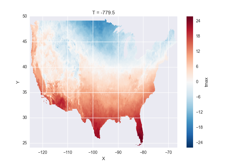
We can select and slice this data any number of times, and nothing is loaded over the network until we look at particular values:
In [16]: tmax = remote_data['tmax'][:500, ::3, ::3]

In [17]: tmax
Out[17]:
<xarray.DataArray 'tmax' (T: 500, Y: 207, X: 469)>
[48541500 values with dtype=float64]
Coordinates:
  * Y        (Y) float32 49.9167 49.7917 49.6667 49.5417 49.4167 49.2917 ...
  * X        (X) float32 -125.0 -124.875 -124.75 -124.625 -124.5 -124.375 ...
  * T        (T) float32 -779.5 -778.5 -777.5 -776.5 -775.5 -774.5 -773.5 ...
Attributes:
    pointwidth: 120
    standard_name: air_temperature
    units: Celsius_scale
    expires: 1443657600

# the data is downloaded automatically when we make the plot
In [18]: tmax[0].plot()
Formats supported by PyNIO
xarray can also read GRIB, HDF4 and other file formats supported by PyNIO,
if PyNIO is installed. To use PyNIO to read such files, supply
engine='pynio' to open_dataset().
We recommend installing PyNIO via conda:
conda install -c dbrown pynio
Formats supported by Pandas
For more options (tabular formats and CSV files in particular), consider exporting your objects to pandas and using its broad range of IO tools.
Combining multiple files
NetCDF files are often encountered in collections, e.g., with different files
corresponding to different model runs. xarray can straightforwardly combine such
files into a single Dataset by making use of concat().
Note
Version 0.5 includes support for manipulating datasets that
don’t fit into memory with dask. If you have dask installed, you can open
multiple files simultaneously using open_mfdataset():
xr.open_mfdataset('my/files/*.nc')
This function automatically concatenates and merges multiple files into a single xarray dataset. It is the recommended way to open multiple files with xarray. For more details, see Reading and writing data and a blog post by Stephan Hoyer.
For example, here’s how we could approximate MFDataset from the netCDF4
library:
from glob import glob
import xarray as xr

def read_netcdfs(files, dim):
    # glob expands paths with * to a list of files, like the unix shell
    paths = sorted(glob(files))
    datasets = [xr.open_dataset(p) for p in paths]
    combined = xr.concat(dataset, dim)
    return combined

combined = read_netcdfs('/all/my/files/*.nc', dim='time')
This function will work in many cases, but it’s not very robust. First, it never closes files, which means it will fail one you need to load more than a few thousands file. Second, it assumes that you want all the data from each file and that it can all fit into memory. In many situations, you only need a small subset or an aggregated summary of the data from each file.
Here’s a slightly more sophisticated example of how to remedy these deficiencies:
def read_netcdfs(files, dim, transform_func=None):
    def process_one_path(path):
        # use a context manager, to ensure the file gets closed after use
        with xr.open_dataset(path) as ds:
            # transform_func should do some sort of selection or
            # aggregation
            if transform_func is not None:
                ds = transform_func(ds)
            # load all data from the transformed dataset, to ensure we can
            # use it after closing each original file
            ds.load()
            return ds

    paths = sorted(glob(files))
    datasets = [process_one_path(p) for p in paths]
    combined = xr.concat(datasets, dim)
    return combined

# here we suppose we only care about the combined mean of each file;
# you might also use indexing operations like .sel to subset datasets
combined = read_netcdfs('/all/my/files/*.nc', dim='time',
                        transform_func=lambda ds: ds.mean())
This pattern works well and is very robust. We’ve used similar code to process tens of thousands of files constituting 100s of GB of data.