You can run this notebook in a live session ![]() or view it on Github.
or view it on Github.
GRIB Data Example
GRIB format is commonly used to disseminate atmospheric model data. With Xarray and the cfgrib engine, GRIB data can easily be analyzed and visualized.
[1]:
import xarray as xr
import matplotlib.pyplot as plt
To read GRIB data, you can use xarray.load_dataset. The only extra code you need is to specify the engine as cfgrib.
[2]:
ds = xr.tutorial.load_dataset('era5-2mt-2019-03-uk.grib', engine='cfgrib')
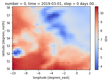
Let’s create a simple plot of 2-m air temperature in degrees Celsius:
[3]:
ds = ds - 273.15
ds.t2m[0].plot(cmap=plt.cm.coolwarm)
[3]:
<matplotlib.collections.QuadMesh at 0x7fef59e462e0>
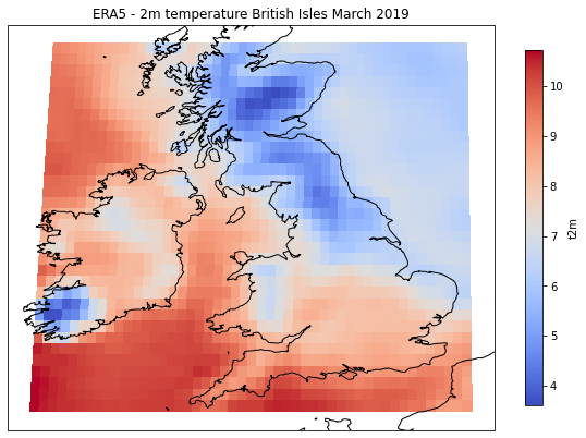
With CartoPy, we can create a more detailed plot, using built-in shapefiles to help provide geographic context:
[4]:
import cartopy.crs as ccrs
import cartopy
fig = plt.figure(figsize=(10,10))
ax = plt.axes(projection=ccrs.Robinson())
ax.coastlines(resolution='10m')
plot = ds.t2m[0].plot(cmap=plt.cm.coolwarm, transform=ccrs.PlateCarree(), cbar_kwargs={'shrink':0.6})
plt.title('ERA5 - 2m temperature British Isles March 2019')
[4]:
Text(0.5, 1.0, 'ERA5 - 2m temperature British Isles March 2019')
/home/docs/checkouts/readthedocs.org/user_builds/xray/conda/v0.17.0/lib/python3.8/site-packages/cartopy/io/__init__.py:260: DownloadWarning: Downloading: https://naciscdn.org/naturalearth/10m/physical/ne_10m_coastline.zip
  warnings.warn('Downloading: {}'.format(url), DownloadWarning)
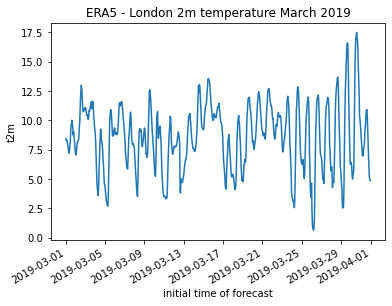
Finally, we can also pull out a time series for a given location easily:
[5]:
ds.t2m.sel(longitude=0,latitude=51.5).plot()
plt.title('ERA5 - London 2m temperature March 2019')
[5]:
Text(0.5, 1.0, 'ERA5 - London 2m temperature March 2019')